Working with data

Data wrangling

Roland Krause

27 November 2025

Introduction - State of the data

During the course of doing data analysis and modeling, a significant amount of time is spent on data preparation: loading, cleaning, transforming, and rearranging. Such tasks are often reported to take up 80% or more of an analyst’s time.

Wes McKinney: Python for Data Analysis - Chapter 7: Data cleaning

On day 1 we started to explore our data, but we did so within the bounds of the data as we found it. That is, we did not change or modify our data in any way. Now we will introduce functions that will allow us to modify our data, starting out with very simple tasks and building towards more complex transformations.

Learning objectives

• Understand what is meant by data wrangling.
• Learn the fundamentals of processing data and preparing data for analysis.
• Become comfortable with the main dplyr functions.
• Practice data wrangling.

Data wrangling

“Data wrangling” refers to the process of taking messy, disorganised, or otherwise unready data and preparing it for downstream analysis.

Data wrangling

Common examples of data wrangling include:

• Renaming variables (columns) such that they all follow a convention.
  E.g., from “winning” and “Loss” to “win” and “loss”.
• Removing NAs.
• Ordering rows or columns.
  E.g., to rank p.values or to sort samples alphabetically)
• Filtering (removing) rows or columns, either based on Boolean operators or to remove duplicates. E.g., keep values > x
• Calculating new, useful values.
  E.g., success_rate = win/loss

All of the above can be completed with a small number of functions from the dplyr package.

The dplyr verbs

Functions for rows:

arrange()

filter()

distinct()

Functions for columns:

relocate()

select()

rename()

mutate()

You will use these dplyr verbs a lot - so we are going to really stress these, and we have exercises for you to practice. Some of these exercises will feel a little repetitive, and that’s deliberate - it’s how we learn.

The dplyr verbs have functional names

arrange() and relocate() change the order of rows and columns.

filter() and select() keep or remove rows and columns.

distinct() returns only unique rows (removes duplicates).

rename() changes the name of a column.

mutate() creates a new variable based on one or more other columns.

Arranging the order

The arrange() function (for rows) and the relocate() function (for columns) allow us to re-order our data.

Note

Rows and columns are not just different axis. Columns have a particular type (numeric, character, time), row are observations that combine different types of data.

arrange() the rows

Start by looking at our data:

penguins |> head()

  species    island bill_len bill_dep flipper_len body_mass    sex year
1  Adelie Torgersen     39.1     18.7         181      3750   male 2007
2  Adelie Torgersen     39.5     17.4         186      3800 female 2007
3  Adelie Torgersen     40.3     18.0         195      3250 female 2007
4  Adelie Torgersen       NA       NA          NA        NA   <NA> 2007
5  Adelie Torgersen     36.7     19.3         193      3450 female 2007
6  Adelie Torgersen     39.3     20.6         190      3650   male 2007

arrange() the rows

penguins |> arrange(body_mass) |> head()

    species    island bill_len bill_dep flipper_len body_mass    sex year
1 Chinstrap     Dream     46.9     16.6         192      2700 female 2008
2    Adelie    Biscoe     36.5     16.6         181      2850 female 2008
3    Adelie    Biscoe     36.4     17.1         184      2850 female 2008
4    Adelie    Biscoe     34.5     18.1         187      2900 female 2008
5    Adelie     Dream     33.1     16.1         178      2900 female 2008
6    Adelie Torgersen     38.6     17.0         188      2900 female 2009

arrange() in descending order

penguins |> arrange(desc(body_mass)) |> head()

  species island bill_len bill_dep flipper_len body_mass  sex year
1  Gentoo Biscoe     49.2     15.2         221      6300 male 2007
2  Gentoo Biscoe     59.6     17.0         230      6050 male 2007
3  Gentoo Biscoe     51.1     16.3         220      6000 male 2008
4  Gentoo Biscoe     48.8     16.2         222      6000 male 2009
5  Gentoo Biscoe     45.2     16.4         223      5950 male 2008
6  Gentoo Biscoe     49.8     15.9         229      5950 male 2009

arrange() the rows

Penguin body mass by year

penguins |> arrange(desc(year),desc(body_mass)) |> head()

  species island bill_len bill_dep flipper_len body_mass  sex year
1  Gentoo Biscoe     48.8     16.2         222      6000 male 2009
2  Gentoo Biscoe     49.8     15.9         229      5950 male 2009
3  Gentoo Biscoe     55.1     16.0         230      5850 male 2009
4  Gentoo Biscoe     50.4     15.7         222      5750 male 2009
5  Gentoo Biscoe     49.5     16.1         224      5650 male 2009
6  Gentoo Biscoe     50.8     17.3         228      5600 male 2009

Combining arguments within the arrange() function can be used for splitting ties (e.g., when you have samples with year, month and date recorded).

Note

You can apply desc() to any number of arguments within arrange(), but you must apply desc() to each variable individually.

Practical uses with arrange()

count() plus arrange() is one way to view the frequency of data.

Exercise: pipe penguins to count(), choosing a single variable to include inside count(), then pipe to arrange().

• Solution: penguins |> count(island) |> arrange(n)

• Why n? Look at the result of penguins |> count(island) and check the variable names.

relocate() the columns

Change the order of columns with relocate().

relocate() takes a column name and moves it to another position in the dataset, defaulting to moving the specified column to the start (left) of the dataset.

penguins |> relocate(year) |> head()

  year species    island bill_len bill_dep flipper_len body_mass    sex
1 2007  Adelie Torgersen     39.1     18.7         181      3750   male
2 2007  Adelie Torgersen     39.5     17.4         186      3800 female
3 2007  Adelie Torgersen     40.3     18.0         195      3250 female
4 2007  Adelie Torgersen       NA       NA          NA        NA   <NA>
5 2007  Adelie Torgersen     36.7     19.3         193      3450 female
6 2007  Adelie Torgersen     39.3     20.6         190      3650   male

relocate() the columns

We can choose to place a column immediately before, or immediately after, another column.

penguins |> relocate(year, .after = island) |> head()

  species    island year bill_len bill_dep flipper_len body_mass    sex
1  Adelie Torgersen 2007     39.1     18.7         181      3750   male
2  Adelie Torgersen 2007     39.5     17.4         186      3800 female
3  Adelie Torgersen 2007     40.3     18.0         195      3250 female
4  Adelie Torgersen 2007       NA       NA          NA        NA   <NA>
5  Adelie Torgersen 2007     36.7     19.3         193      3450 female
6  Adelie Torgersen 2007     39.3     20.6         190      3650   male

(Re)arranging summary

Remember: arrange is for rows, while select is for columns.

arrange() is functionally sorting rows, while select() is a manual re-organising of columns.

Reminder: none of our functions are modifying the original dataset. Re-arranged data is only being displayed on the screen. Save the output of these functions to a new object if you want to store data.

It’s your turn!

Order and rearrange

1. Arrange the penguins in order of body mass (lightest to heaviest).

2. Arrange the penguins by flipper length, with the longest flippers first.

3. Within each species, sort penguins by bill length.

4. Move all the measurement columns so they appear immediately after species.

5. Move the year column so that it appears last.

 

Challenge: Create a table that lists penguins ordered by body mass (heaviest first) with the species and measurement columns shown first.

Keeping or removing data

The next two functions are filter() (for rows) and select() (for columns).

In both cases we will specify which data to keep and the rest will be discarded.

As above, we can use the r in filter and the c in select to help us remember which function is rows and which is for columns.

filter() with single criteria

Keep all rows that meet a certain criteria in a given column. Criteria can be built using any combination of Boolean values (greater than, less than or equal to, exactly equal to) using “and” or “or” e.g., keep any row if the value is greater than 1 or less than -1

penguins |> filter(body_mass > 4000) |> head()

  species    island bill_len bill_dep flipper_len body_mass  sex year
1  Adelie Torgersen     39.2     19.6         195      4675 male 2007
2  Adelie Torgersen     42.0     20.2         190      4250 <NA> 2007
3  Adelie Torgersen     34.6     21.1         198      4400 male 2007
4  Adelie Torgersen     42.5     20.7         197      4500 male 2007
5  Adelie Torgersen     46.0     21.5         194      4200 male 2007
6  Adelie     Dream     39.2     21.1         196      4150 male 2007

filter() combinations

penguins |> filter(body_mass > 4000) |> count()

    n
1 172

penguins |> filter(body_mass > 4750) |> distinct(island)

  island
1 Biscoe
2  Dream

Chaining together functions like this is very powerful!

Filter criteria

• > return all values greater than x

• < return all values less than x

• >= return all values greater than or equal to x

• == return all values exactly equal to

filter() with and/or

penguins |> filter(species == "Gentoo" & bill_len > 50) |> count()

   n
1 22

22 Gentoo samples have a bill length greater than 50.

penguins |> filter(species == "Gentoo" | island == "Biscoe") |> count()

    n
1 168

168 samples are either Gentoo species OR are found on the Biscoe island.

It’s your turn!

filter() practice

1. How many Adelie penguins are there?

2. Using a single command, show which island has the most penguins.

3. Display all the Gentoo penguins which have a body mass greater than 5000g.

4. For how many penguins do we have sex data?

5. I define a small penguin as weighing less than 3500g and having a bill shorter than 35mm. How many penguins meet this criteria?

select() the columns to keep

select() defines which columns are kept.

penguins |> select(species, island) |> head()

  species    island
1  Adelie Torgersen
2  Adelie Torgersen
3  Adelie Torgersen
4  Adelie Torgersen
5  Adelie Torgersen
6  Adelie Torgersen

Keeping a range of columns

penguins |> select(bill_len:body_mass) |> head()

  bill_len bill_dep flipper_len body_mass
1     39.1     18.7         181      3750
2     39.5     17.4         186      3800
3     40.3     18.0         195      3250
4       NA       NA          NA        NA
5     36.7     19.3         193      3450
6     39.3     20.6         190      3650

select() advanced usage

Here we will demonstrate a powerful feature of programming languages: the ability to perform pattern matching. Pattern matching is not covered in this course, but consider this a gentle introduction to the concept.

Instead of needing to select individual variables we can select variables that meet a criteria, such as “starts with the letter b” or “contains an _“.

select() advanced usage

penguins |> select(starts_with("bill")) |> head()

  bill_len bill_dep
1     39.1     18.7
2     39.5     17.4
3     40.3     18.0
4       NA       NA
5     36.7     19.3
6     39.3     20.6

penguins |> select(ends_with("s")) |> head()

  species body_mass
1  Adelie      3750
2  Adelie      3800
3  Adelie      3250
4  Adelie        NA
5  Adelie      3450
6  Adelie      3650

select() advanced usage

penguins |> select(contains("_")) |> head(n = 4)

  bill_len bill_dep flipper_len body_mass
1     39.1     18.7         181      3750
2     39.5     17.4         186      3800
3     40.3     18.0         195      3250
4       NA       NA          NA        NA

select() everything except

Do not select species, but keep everything else.

penguins |> select(!species) |> head(n = 4)

     island bill_len bill_dep flipper_len body_mass    sex year
1 Torgersen     39.1     18.7         181      3750   male 2007
2 Torgersen     39.5     17.4         186      3800 female 2007
3 Torgersen     40.3     18.0         195      3250 female 2007
4 Torgersen       NA       NA          NA        NA   <NA> 2007

Tip

Use !contains() to exclude variables containing a specific pattern.

It’s your turn!

Combining arguments

This exercise will reinforce your understanding of combining arguments.

Use select() and starts_with() to keep all columns that measure a physical feature of the penguins (bill_len, bill_dep, flipper_len, body_mass).

Code we have used today which might help:

select(starts_with("bill"))

filter(species == "Gentoo" | island == "Biscoe")

Solution

You may have tried this:

penguins |> select(starts_with(“b” | “f”)) |> head()

We need to specify starts_with() for each criteria individually. We used this same logic earlier when we used arrange(desc(year),desc(body_mass)).

penguins |> select(starts_with("b") | starts_with("f")) |> head()

  bill_len bill_dep body_mass flipper_len
1     39.1     18.7      3750         181
2     39.5     17.4      3800         186
3     40.3     18.0      3250         195
4       NA       NA        NA          NA
5     36.7     19.3      3450         193
6     39.3     20.6      3650         190

Understanding the solution

This gives us more precise control over our criteria.

e.g., what if you needed to specify starts with b or ends with f?

Initially, starts_with("b" | "f") seems logical. It sounds right: “Starts with b or f”. However, when we imagine a more complex example, like if we needed to specify starts with b or ends with f, or starts with A and contains an underscore, we can see it is logical to specify each criteria individually.

distinct() to remove duplicate rows

The distinct function will remove rows that have the same value for a selected criteria.

penguins |> distinct(year) |> head()

  year
1 2007
2 2008
3 2009

All duplicates of “2007”, “2008”, “2009” have been removed.

Unique combinations

penguins |> distinct(species, island)

    species    island
1    Adelie Torgersen
2    Adelie    Biscoe
3    Adelie     Dream
4    Gentoo    Biscoe
5 Chinstrap     Dream

 

Reveals Adelie penguins are found on all three islands, while Gentoo and Chinstrap are restricted to Biscoe and Dream, respectively.

It’s your turn!

Combining filter and distinct for complex tasks

For each penguin species, identify which islands they are found on.

Filter for penguins with a body mass greater than 4000g, then find the distinct species-sex combinations (e.g., among ‘big’ penguins, are there both males and females from all species, or are only some species/sexes present).

Filter for Gentoo penguins from the Biscoe island. How many distinct years were they sampled in?

mutate() calculates new variables

mutate() takes information from one or more columns and creates a new variable which is immediately added to the object.

penguins |> 
  mutate(bill_dim_ratio = bill_len / bill_dep) |> 
  arrange(desc(bill_dim_ratio)) |> 
  select(contains("_")) |> 
  head()

  bill_len bill_dep flipper_len body_mass bill_dim_ratio
1     51.3     14.2         218      5300       3.612676
2     50.2     14.3         218      5700       3.510490
3     59.6     17.0         230      6050       3.505882
4     46.1     13.2         211      4500       3.492424
5     54.3     15.7         231      5650       3.458599
6     48.7     14.1         210      4450       3.453901

mutate() has calculated a new variable called bill_dim_ratio (bill dimension ratio) based on the formula we provided and data from those variables.

Data has been arranged based on this new variable (note, it’s immediately available, you don’t have to ouput this data somewhere before you can interact with the new variable.)

select() used to reduce the number of columns on the screen.

It’s your turn!

mutate() some new variables

1. Create a new variable called body_mass_kg.

2. Create a new variable flipper_to_mass_ratio, and sort it in decreasing order. - This is called a derived variable and is extremely useful.

3. Create a new variable called heavy indicating whether body_mass is greater than 4.5kg.

mutate() and case_when()

case_when() is useful for adding ‘class’ variables.

penguins |> 
  mutate(flipper_class = case_when(
    flipper_len < 190 ~ "short",
    flipper_len <= 210 ~ "medium",
    TRUE ~ "long"
  )) |> 
  distinct(species, flipper_class)

    species flipper_class
1    Adelie         short
2    Adelie        medium
3    Adelie          long
4    Gentoo          long
5    Gentoo        medium
6 Chinstrap        medium
7 Chinstrap         short
8 Chinstrap          long

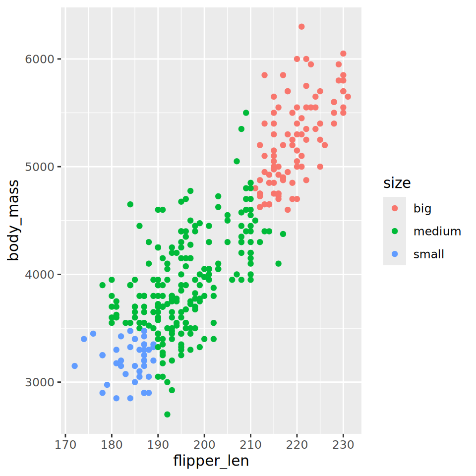
case_when() combines well with ggplot

Use case_when() to define penguins as ‘big’, ‘medium’ or ‘small’ based on two variables (this is arbitrary, you decide how to define these values). Call the new variable “size”.

Recall the code for ggplot, and generate a plot showing the two variables on the x and y axis, with size shown by colour.

• Hint: the code for case_when(): mutate(flipper_class = case_when( flipper_len < 190 ~ “short”, flipper_len <= 210 ~ “medium”, TRUE ~ “long” ))

Solution

penguins |> 
  mutate(size = case_when(
    flipper_len > 210 & 
      body_mass > 4500 ~ "big",
    flipper_len < 190 & 
      body_mass < 3500 ~ "small",
    TRUE ~ "medium"
  )) |> 
  ggplot(mapping = aes(x = flipper_len,
                       y = body_mass,
                       colour = size)) +
  geom_point()

rename() columns

rename() renames variables.

Keep variable names short, descriptive, and uniform.

Develop a system and be consistent.

We strongly recommend that all objects and files are named in snake_case.

all_people_like_snake_case

penguins |> rename(f_len = flipper_len) |> head()

  species    island bill_len bill_dep f_len body_mass    sex year
1  Adelie Torgersen     39.1     18.7   181      3750   male 2007
2  Adelie Torgersen     39.5     17.4   186      3800 female 2007
3  Adelie Torgersen     40.3     18.0   195      3250 female 2007
4  Adelie Torgersen       NA       NA    NA        NA   <NA> 2007
5  Adelie Torgersen     36.7     19.3   193      3450 female 2007
6  Adelie Torgersen     39.3     20.6   190      3650   male 2007

group_by()

So far we have calculated summary statistics or arranged our data assuming all our observations are homogeneous, i.e., we have not dealt with sub-groups.

How do we calculate the mean body mass by species, island, or sex?

group_by() allows us to move from computing a single summary statistic to calculating multiple summary statistics.

group_by() is functionally tagging observations with group labels.

Mechanics of group_by()

# Looks the same
# Note "Groups: species [3]"
penguins |> group_by(species)

# A tibble: 344 × 8
# Groups:   species [3]
   species island    bill_len bill_dep flipper_len body_mass sex     year
   <fct>   <fct>        <dbl>    <dbl>       <int>     <int> <fct>  <int>
 1 Adelie  Torgersen     39.1     18.7         181      3750 male    2007
 2 Adelie  Torgersen     39.5     17.4         186      3800 female  2007
 3 Adelie  Torgersen     40.3     18           195      3250 female  2007
 4 Adelie  Torgersen     NA       NA            NA        NA <NA>    2007
 5 Adelie  Torgersen     36.7     19.3         193      3450 female  2007
 6 Adelie  Torgersen     39.3     20.6         190      3650 male    2007
 7 Adelie  Torgersen     38.9     17.8         181      3625 female  2007
 8 Adelie  Torgersen     39.2     19.6         195      4675 male    2007
 9 Adelie  Torgersen     34.1     18.1         193      3475 <NA>    2007
10 Adelie  Torgersen     42       20.2         190      4250 <NA>    2007
# ℹ 334 more rows

Can group by more than one variable e.g., group_by(species, island)

Combining group_by() with other functions

group_by() plus another function will cause that function to be applied to individual groups (e.g., returning summary statistics, arranging, or filtering on a per-group basis).

penguins |> 
  group_by(species) |> 
  summarize(mean_body_mass = mean(body_mass, na.rm = TRUE))

# A tibble: 3 × 2
  species   mean_body_mass
  <fct>              <dbl>
1 Adelie             3701.
2 Chinstrap          3733.
3 Gentoo             5076.

Exercise: Change group_by() to group by species and island and note the output.

group_by and filter()

Find the heaviest penguin per species:

penguins |> 
  group_by(species) |> 
  filter(body_mass == max(body_mass, na.rm = TRUE))

# A tibble: 3 × 8
# Groups:   species [3]
  species   island bill_len bill_dep flipper_len body_mass sex    year
  <fct>     <fct>     <dbl>    <dbl>       <int>     <int> <fct> <int>
1 Adelie    Biscoe     43.2     19           197      4775 male   2009
2 Gentoo    Biscoe     49.2     15.2         221      6300 male   2007
3 Chinstrap Dream      52       20.7         210      4800 male   2008

A preview of tomorrow

ggplot(
  data = penguins,
  mapping = aes(x = bill_len,
                y = bill_dep,
                shape = island, 
                colour = species)) +
  geom_point()

With just a few lines of code we can produce a plot like this. Cool, right??? No! This is a hideous, terrible plot that should never be seen in public. I mean, it’s fine if I want to check something quickly, but look at it. No title, ugly axis labels, horrible colour scheme. Tomorrow, we will learn how to make plots to be proud of.

But first …

Installation and setup of git

Git helps to version and share code.