Introduction to R and RStudio

Getting started with R

26 November 2025

This workshop…

Assumes you are an absolute beginner.

Will teach you the fundamentals of working in R by walking through a ‘typical’ bioinformatics workflow.

We will work slowly and there will be repetition. You will build good habits through experience.

At the end of this course you will grasp the fundamentals and be in a good position to work with google, llms, supervisors and colleagues to solve specific problems and challenges.

Workshop aims

We will:

• Set up a new Project in RStudio to help manage all our files.

• Import data into RStudio.

• Clean and tidy the data.

• Visualise the data for ourselves.

• Carry out “data wrangling” (getting the data into the shapes and formats we need).

• Visualise the data for presentation.

Objectives for the course

• Learn how to use RStudio and Projects to keep work organised.

• Learn the fundamentals of the R programming language: functions, objects and packages.

• Develop the habit of writing readable, reproducible code.

• Be able to interpret errors and warnings.

• Understand the format of data in R.

• Use the dplyr functions for data preparation and processing (“wrangling”).

• Be able to create basic visualisations of your data.

On the topic of LLMS

Many llms write very good R code if given accurate context and clear requests.

Many llms will struggle to solve the issues you encounter in R because you don’t know what the issue is.

During this workshop, please refrain from using llms to solve exercises. You need to practice doing these tasks.

The R programming language

• Created in 1993 by Dr. Ross Ihaka and Dr. Robert Gentleman at the University of Auckland, Aotearoa New Zealand.
• Widely used in statistics and biological sciences.
• Free, flexible, supported by the community.
• Base R was used to build packages that accomplish specific tasks.
• Base R packages includes a mix of styles and formats.
  • Challenging to learn!

The tidyverse dialect

• A series of packages designed from the ground up to work together.
• Uses a consistent and logical style with a shared format.
• Human readable, intuitive, easy to learn.
• Highly popular, well documented, many resources available.
• Designed by programmers for non-programmers.

The tidyverse style

Each variable stored in a column.

Each observation is stored in a row.

penguins[1:3,1:6]

  species    island bill_len bill_dep flipper_len body_mass
1  Adelie Torgersen     39.1     18.7         181      3750
2  Adelie Torgersen     39.5     17.4         186      3800
3  Adelie Torgersen     40.3     18.0         195      3250

The RStudio interface

RStudio is an interface for R.

Analogy: R is the engine, RStudio is driver’s seat.

When you first open RStudio it will look something like this image. Right now there are three panes or windows: Console which is where our code gets run, Environment which is where we see what data we have in RStudio, and Files which is showing us files on our computer. We can also see that each of these windows has different tabs. E.g., Files pane also has Plots, Packages, Help, and others.

The first thing we are going to do is to customize our RStudio.

Customising RStudio: adding a source pane

It is best practice to write all code in a document to be saved.

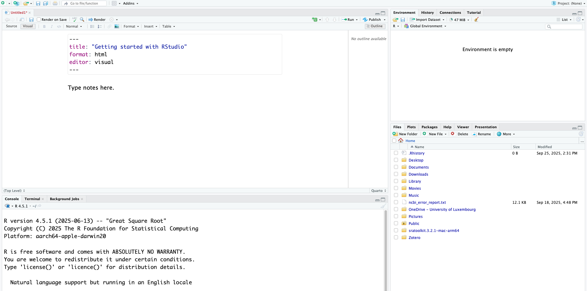
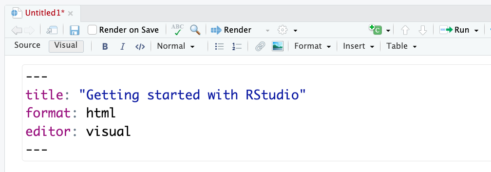
Click File > New File > Quarto Document.

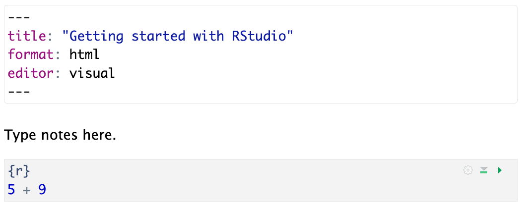
Give this file the title: “Getting started with RStudio” and click “Create Blank Document” on the bottom left.

We will use this new space to write our code and our notes.

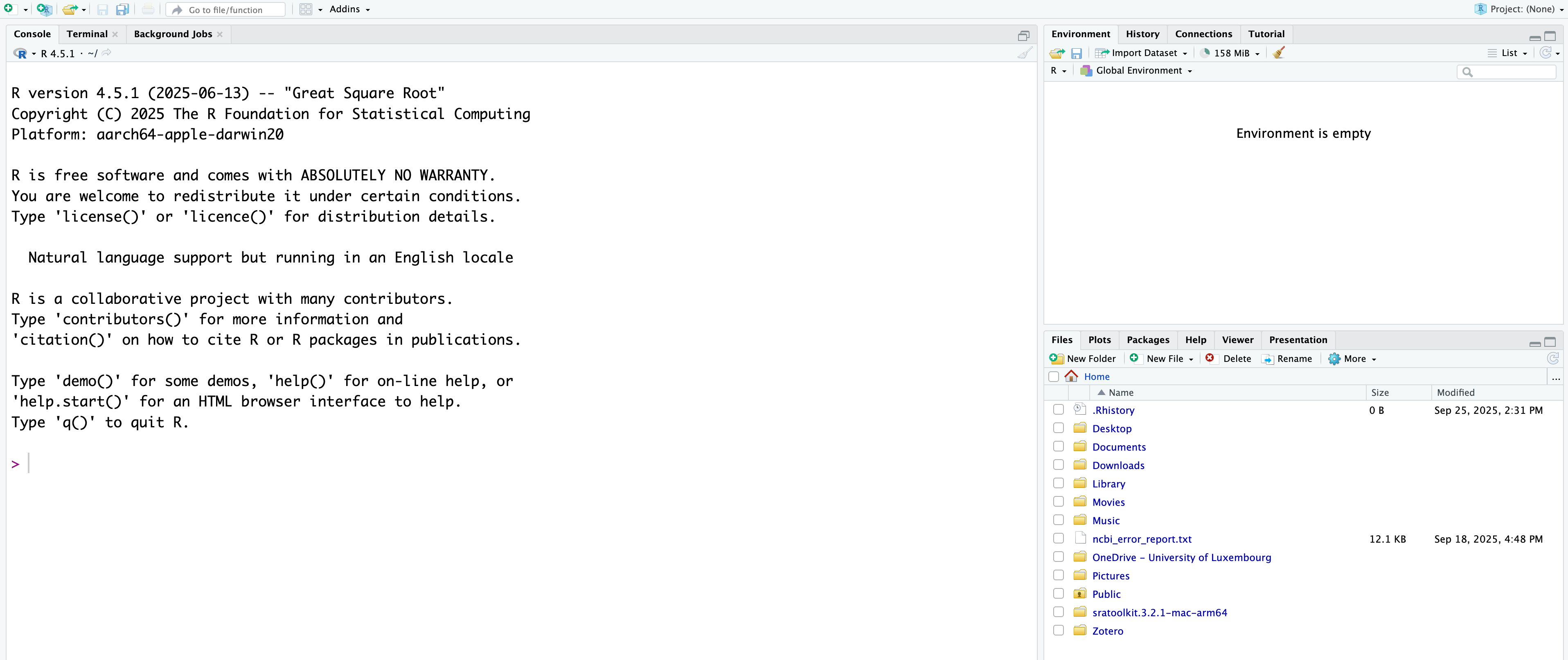
Your screen should now look like this:

We will cover writing in this document, which is called an R script or Quarto document, in more detail soon. For now, the key thing to remember is that we always want to write our code in this document.

Customising the RStudio layout

We can rearrange the layout of the four panes.

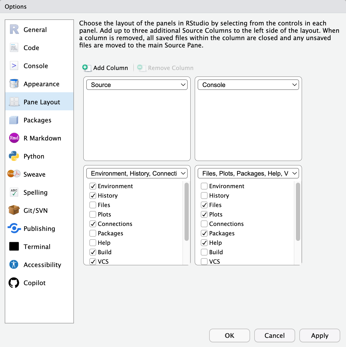
Click Tools > Global Options to bring up the options window.

Select the “Pane Layout” tab, and use the drop-down arrows to set the four panes to be Source, Console, Environment, and Files.

In this section we will rearrange the four panes (windows) into a common configuration. Many people seem to prefer this layout over the default, so we recommend you adopt this while you are getting started.

Let’s write and run some R code

We will write and run code directly from the source document we just opened.

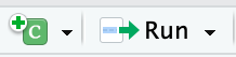
We store all code in “chunks”. To add a chunk, click on the button that looks like a green square with a white “C”, and a small green “+” in the top left. It should be to the left of the “Run” button.

Code chunks

Within the code chunk, type some basic arithmetic (e.g., 5 + 9).

Run the chunk with the green arrow on the right.

Code chunks cont

We should see the code and the output appear in the console.

This is how we work in R: write code in a document, run the code, output is either displayed on the screen or saved as files.

It’s your turn!

Buttons are slow - use shortcuts!

Use either option + command + i (Mac) or Ctrl + Alt + i (Windows) to add a new code chunk.

In the new chunk write:

6 + 6

[1] 12

4 * 12

[1] 48

Click anywhere on the line that says 6 + 6 and use command + return (Mac) or Ctrl + enter to run the code.

Save the file so that this code can be accessed later.

You can either run all the code within a chunk with the green arrow, OR you can highlight all the code in the chunk and use command+return / ctrl+enter.

You can put the mouse cursor anywhere on a line to execute it - it does not have to be at the start or the end.

New users waste so much time carefully highlighting, or moving the mouse around, just to run code!

Similarly, use the keyboard shortcuts for copy paste. Do not right click and select “copy”.

After saving, ask everyone to close the script.

Group discussion about files

• Where did you save your file?

• What did you call your file?

• Can you locate that file on your device right now?

Start with poll: hands up if you saved this file to your desktop, to Downloads, to Documents. Hands up if you have a lot of random files saved in this location.

Did anyone save it somewhere carefully?

File naming poll: hands up if you named your file some combination of “file”, “r”, “script”, “quarto”, “final.final”.

Ask audience to share what they called their files.

Poll: Using an explorer browser (finder on Mac, Explorer on Windows) who can find their file?

File locations and names

Modern devices (including most Apple products) automatically store files and make them available as “Recent documents”.

Result: we don’t need to think about where our files are going.

In bioinformatics we need to think about where our files are at all times.

Projects

RStudio uses “Projects” to manage files.

Use one project per topic:

• This workshop should be one project.

• An assignment for a paper would be one project.

• A thesis, dissertation, or book would be one project.

In the next section we will demonstrate how to set up a project.

Projects cont: what is a project?

Projects keep your work together and organised.

Each project is self-contained and portable.

Sets your working directory and controls file paths.

Practically: a project is a single directory with a .Rproj file that manages how RStudio interacts with other files you are working with.

Practically, a project is a way to automate most of the work involved in saving files in the right place, and making sure we can access files. We will see later that when you want to import data into RStudio we need to tell RStudio where the file is found, and we need to use very clear and specific language when we do that. Projects will make this process much easier.

An analogy would be to say we are dedicating a single box or drawer in our desk to a topic. Every time I find something, or make something, that relates to my topic it goes in the one drawer, AND, I have a list of all the things that are in the drawer.

Starting a Project in RStudio (Demonstration)

Watch while the instructor creates a new project.

File > New Project > New Directory > New Project

Set Directory name to “intro_to_r”. Create project as a subdirectory of ~/Documents.

Select Create Project.

RStudio will re-start.

For now, just watch the process and listen to the instructions. We will walk you through doing this as a group in the next slide. For now, just watch and listen.

Switch to RStudio, demonstrate setting up new project.

It’s your turn!

Start a new project

• Set Directory name to “intro_to_r”.

• Create project as a subdirectory of ~/Documents.

• Look for the “intro_to_r.Rproj” file in the files Pane.

• Open a new Quarto document (File > New File), call it “Day 1” and save it as “day_1.qmd”.

• RStudio should default to saving day_1.qmd to your project directory.

Give students a 2-5 minute head start, checking in with the audience. Encourage people to discuss with others. Invite questions.

Walk through the process from start to finish, demonstrating the process.

Reiterate: “intro_to_r” is a folder that exists on our machine. We need to be able to find it, and from now on we will make sure we save everything relating to this project in here. If we have some raw data, we will put a copy in here, if we make some figures they will get saved to here.

Customising RStudio

RStudio has many user options.

We will use Global Options to set ‘soft wrap’, the native pipe, and set an editor theme.

Before doing Tools > Global options, ask that students do NOT follow, and only watch. Under Code, tick soft wrap and native pipe. Under appearance set an editor theme. Mention some examples of high-intensity (e.g., Gob) and gentle options (Chrome).

Then ask students to repeat what you did. This gives them an opportunity to explore the Global Options menu by memory and reinforces the process + the skill of finding buttons.

Follow me!

Let’s customise our RStudio interface

It’s your turn!

Exercise: Customise your RStudio

• Under Tools (to the right of File), select Global Options.

• In the Code tab, tick “Soft-wrap source files”.

• In the Appearance tab:

  • Adjust the Editor font size and Editor font to suit you (the default font is Monaco).

  • Choose an Editor theme. You will spend a long time looking at your RStudio screen, we recommend something with high contrast that is not too hard to look at. Try these examples:

    • Chrome, Crimson Editor and Dreamweaver are gentle light themes.

    • Cobalt, Idle Fingers and Pastel on Dark are gentle dark themes.

    • What is your opinion on the Gob editor theme?

Project wrap-up

What questions do you have about projects?

An opportunity for questions or discussion.

Note that from here we are about to pivot into actually working with RStudio and some example data. It’s important to get these foundations set.

The bioinformatician’s workflow

Almost any project will include the following steps:

• Import data

• Exploratory analysis

• Data wrangling

• Visualisations and other outputs

R is a language. Most workshops, in my experience, focus on the basics. They explain that R uses functions to do stuff, objects for storing information, and then talk about all the different ways that we can store data and how exactly a function works.

In this workshop we are going to take a different approach and will dive straight into more complicated stuff. The idea is that you will learn the basics by doing. As an analogy, I’m learning French right now and we didn’t start with liaisons. We started with some basic questions and answers, and the specific details like liaisons are thrown in as they come up.

Almost any project will contain four major steps: importing data, exploring the data, modifying or wrangling the data, and creating some finished product - often a visualisation. We will work through this basic format today.

Importing data

R is primarily used for handling ‘flat’ data: rows and columns.

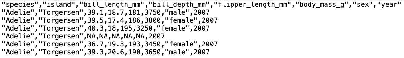
The most common type of flat data file is the CSV (comma separated values).

Typically, the first row will contain column names and is referred to as the “header”. Rows underneath the header contain data for each column, with columns separated by commas.

The csv format

Importing data: setting up

First, store the data within a /data subdirectory.

Second, install and load packages for importing data.

Inform the audience that the installing, loading, and importing is how we will first look at two key features of R: functions and objects. Functions and objects are the two things we really need to understand in R, but rather than giving you some definitions we will jump into using them.

It’s your turn!

Exercise: storing data

• Go to https://tinyurl.com/penguinData2025. Use the download button to get a local copy of the file.

• In your intro_to_r project directory, create a subdirectory called data.

• Copy/move the penguin_dataset.csv file to the new data directory.

• Then:

• Open a new quarto document with the title “Intro to R Day 1”.

• Save it as day_1.qmd

• Type “## Setup” (this should appear as a heading).

• Type “### Packages”

It’s critical to save keep everything in our project directory, and because it can get big and messy very quickly, we want to keep it organised with sub directories.

Packages

Packages are collections of additional data or functions that extend the R language.

We can equate packages with apps.

To use a package requires two steps:

• Install the package from a remote repository (one-time only)

• Load the package into RStudio (every session)

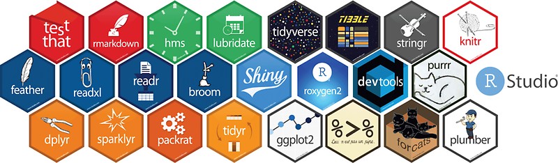
Hex stickers

It’s your turn!

Install and load the tidyverse

Create a code block in your quarto doc, add the code below, and execute:

Install packages - run this the first time you work with a new package.

install.packages("tidyverse")

Load packages - run this every time you work with the package.

library(tidyverse)

Test this with (new code block):

tidyverse_packages()

 [1] "broom"         "conflicted"    "cli"           "dbplyr"       
 [5] "dplyr"         "dtplyr"        "forcats"       "ggplot2"      
 [9] "googledrive"   "googlesheets4" "haven"         "hms"          
[13] "httr"          "jsonlite"      "lubridate"     "magrittr"     
[17] "modelr"        "pillar"        "purrr"         "ragg"         
[21] "readr"         "readxl"        "reprex"        "rlang"        
[25] "rstudioapi"    "rvest"         "stringr"       "tibble"       
[29] "tidyr"         "xml2"          "tidyverse"    

This may be the first time attendees see a function. Highlight the format of verb(target/argument - and sometimes empty). Be very clear that R is fussy, and will not tolerate spaces, capitals, misplaced commas or out-of-sync quotes and brackets. Functions do a massive range of things.

The tidyverse is a package that actually contains a whole lot of other packages. Installing and loading the tidyverse will give you access to example datasets and hundreds of new functions. Here we specifically want a function from the tidyverse for importing data.

Mention the use of hash symbols to comment out information. After running install tidyverse once, I’d then add a hash in front of it.

Importing data

Our project dictates our current working directory. Files must be described relative to the project directory.

The read_csv function:

read_csv(file = "data/penguin_dataset.csv")

Reading the data into an object:

penguins <- read_csv(file = "data/penguin_dataset.csv")

First, don’t type this whole thing. Type “read_” then use the arrows to select read_csv().

Second, we need to provide the exact file for the function. This is probably one of the most challenging parts of getting started with R. We need to understand that because we have set up a project, R is treating the project as our starting point. When specifying the file we should, after opening our quotes, type “da” and use tab-completion. Tab completion is critical for avoiding typos - learn to use it aggressively.

Note on the second line a special case: “<-” this means to take the data and store it inside an object.

After running the second line, we should see something has appeared in our Environment tab. More on this in the next slides:

Functions and objects

• We can think of objects as being equivalent to files.
• Functions do things:
  • Calculate the mean of a series of numbers.
  • Count the number of times a name has appeared in a list.
  • Rename or reorganise columns (variables) in a file.

Objects as equivalent to files - we can see that we have this new object in our environment, and we can see that it contains information, in this case: data about penguins.

If we want to do something with this data we need to use functions.

It’s your turn!

Examine the penguins data object

There are many functions we can use to examine our data. Test these functions and draw some initial conclusions about your data.

penguins |> head()
penguins |> tail()
penguins |> View()
penguins |> summary()
penguins |> colnames()
penguins |> dim()

This new symbol is called the pipe. You should be able to add it with command+shift+m (mac) or cntrl+shift+m (windwos).

Two minutes to look at the penguins data, remind to draw conclusions. Then:

First, note the format. With the exception of View(), all are lowercase, open a round-bracket or parentheses, then type the target. Second, what is the pipe doing? Third, going around the group, what does each function do? Fourth, what can we say about our data?

A small note on functions

We just saw the head() function. head() and tail() print the first, or last, six rows of the object.

head(penguins, 4)

# A tibble: 4 × 8
  species island    bill_len bill_dep flipper_len body_mass sex     year
  <chr>   <chr>        <dbl>    <dbl>       <dbl>     <dbl> <chr>  <dbl>
1 Adelie  Torgersen     39.1     18.7         181      3750 male    2007
2 Adelie  Torgersen     39.5     17.4         186      3800 female  2007
3 Adelie  Torgersen     40.3     18           195      3250 female  2007
4 Adelie  Torgersen     NA       NA            NA        NA <NA>    2007

• Functions can be modified with arguments.

• Most functions have defaults which are not shown. Be aware of function defaults!

The pipe

This works best if you read “|>” as “and then…”

penguins |> # Start with the penguin data AND THEN
  na.omit() |> # Remove the NAs AND THEN
  arrange(bill_len) |>  # Arrange (sort) the rows AND THEN
  head() # Keep just the head (top 6 rows)

# A tibble: 6 × 8
  species island    bill_len bill_dep flipper_len body_mass sex     year
  <chr>   <chr>        <dbl>    <dbl>       <dbl>     <dbl> <chr>  <dbl>
1 Adelie  Dream         32.1     15.5         188      3050 female  2009
2 Adelie  Dream         33.1     16.1         178      2900 female  2008
3 Adelie  Torgersen     33.5     19           190      3600 female  2008
4 Adelie  Dream         34       17.1         185      3400 female  2008
5 Adelie  Torgersen     34.4     18.4         184      3325 female  2007
6 Adelie  Biscoe        34.5     18.1         187      2900 female  2008

With the pipe we can “chain” together functions to achieve complex tasks. Notice how it is still (mostly) readable.

This is generally what we want our code to be. It’s human readable, there is documentation, this block of code is doing one thing. Note the format, the indents, and the use of one function per line.

Write good code

What is good code?

• Strict ‘style’: spaces around operators and commas.

• Objects are named in lowercase and numbers, and use _ to separate.

• One function per line (generally).

• Pipes are at the end of a line and are preceded by spaces. After a pipe, indent (automatic).

• Add comments! Document your work.

Errors and warnings

RStudio will (very) regularly provide you with two types of feedback:

• Errors, which tell you something has failed and must be addressed.
  • Identify the error and change your code.
  • Initially you will make many spelling and typing errors - R is very fussy!
  • Alternatively, find a new approach.

Warnings

• Warnings, which tell something has happened and you should be aware of it.
  • There is a new version of the software you are using.
  • Two packages you are using may contradict one another.
  • NAs were removed or ignored when performing a function.

It’s your turn!

Interpreting errors and warnings

Run the following functions and identify what the problem is and what you need to do to fix it.

library(heatmap)
penguins2 <- read_csv(file = "penguins_dataset.csv")
penguins |> mean(flipper_len)
my_variable <- 0983
my_varıable

Note you don’t have to fix it, just understand what the message is telling you and theoretically what you need to do to fix it.

Sometimes errors are almost incomprehensible. But, they give you something to google. Some errors are complex enough that LLMs will send you in completely the wrong direction, but if you know more about R you can provide enough context that you’ll be able to solve it.

Exploratory analysis

What do you do when you get new data?

Need to understand the format, shape, type.

Are numerical values normally distributed? Are there outliers? Do we have batch effects?

Exploring the penguins dataset

Use the glimpse() function to look at the penguins dataset.

What are the data types of each column? Which are categorical, which are numeric?

Use the count() function on one of the categorical variables.

Beyond numbers and words

“Far better an approximate answer to the right question, which is often vague, than an exact answer to the wrong question…”

      - John Tukey
      

“The simple graph has brought more information to the data analyst’s mind than any other device. It specializes in providing indications of unexpected phenomena”.

      - John Tukey
      

Two quotes. First, a quote on what we are trying to achieve with this section. We want to sketch rough graphs that address very specific, very simple questions. If I squint at the data, can I see groups? Does that sample look like an outlier? Does something ‘feel off’, which sounds not very scientific but it’s a place to start.

Second quote, people often quote the first sentence that the graph brings more information, but I rarely see the second part, which highlights the graph shows us unexpected things. In the course of your career you will, on many occasions, think your data is X and then a graph shows you it’s actually Y (or X + something unknown).

For the rest of the section we are going to use very basic plots to explore our data. We will re-visit plots on our third day and really focus on how to get good quality plots that we can be proud of.

Data visualisation with ggplot

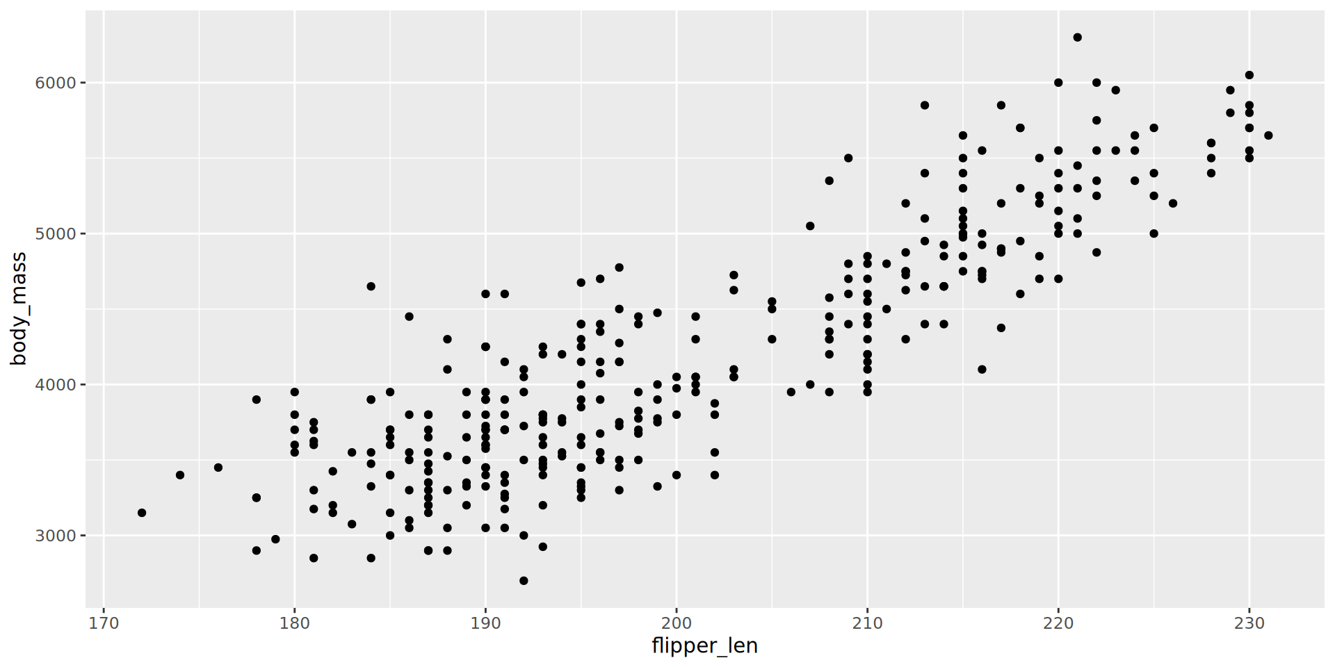
• ggplot (“Grammar of Graphics”): work iteratively, build complexity.

• Focus on the format.

• Demonstrates a key loop in data analysis: visualise your data, make adjustments, transform the data and visualise again.

The ggplot format

The ggplot format has three parts:

Calling the ggplot function and specifying the data.

Mapping the data: what data is displayed on the x and y axis.

Plotting the data with a geom function - there are different geoms for different types of plots.

• Note that the geom is a new function, which means we need to add a “+” to the previous line.

The ggplot format

ggplot(data = penguins, 
       mapping = aes(x = bill_len,
                     y = bill_dep)) +
  geom_point()

Exercise: What do you notice about the format of this code?

• No pipes, instead objects and arguments are all inside the function bracket.

• The “+” and/or there are two functions.

• Comparing bill length and depth.

• The format: indents, alignment, it’s very readable.

Exercise/Discussion: What do you notice about the format of this code? 1. No pipes, instead objects and arguments are all inside the function bracket. 2. The “+” and/or there are two functions. 3. Comparing bill length and depth. 4. The format: indents, alignment, it’s very readable.

The ggplot format

Exercise: Interpret this graph, discuss your observations.

• Does this data fit, approximately, with our expectations?

• Do you observe sub-groups? If so, how many? What is a possible explanation?

This is a nice plot for four lines of code. Automatically set the scale and the axis labels are functional if ugly.

Made the plot. Now what? What’s the first thing we should do?

Whatever we are visualising we should always ask ourselves whether the data makes sense. What do we observe? Does it fit with our expectations and knowledge of the data?

Do I expect bill length and depth to be correlated? Yes, broadly.

What else do you see?

Are there sub-groups? How many? What could be the cause? We will address this question shortly.

It’s your turn!

Exercise: clear your screen of previous code

• From memory, create a new plot using:

  • ggplot(), where data = penguins and

  • mapping = aes() with:

    • flipper_len on the x axis, body_mass on the y axis

  • geom_point()

  • Remember that after the ggplot() function add a “+” before geom_point()

Solution

ggplot(data = penguins,
       mapping = aes(x = flipper_len,
                     y = body_mass)) +
  geom_point()

What variable could explain the groups in this graph?

How do we address this question?

Mapping additional variables

mapping = aes() is used to map a variable to an axis.

Variables can also be mapped to axes other than x and y:

Colour, size, and shape are all axes we can map aesthetics to.

Mapping additional variables

ggplot(data = penguins,
       mapping = aes(x = bill_len,
                     y = bill_dep,
                     colour = sex)) +
  geom_point()

It’s your turn!

Exercise: Explain the sub-grouping

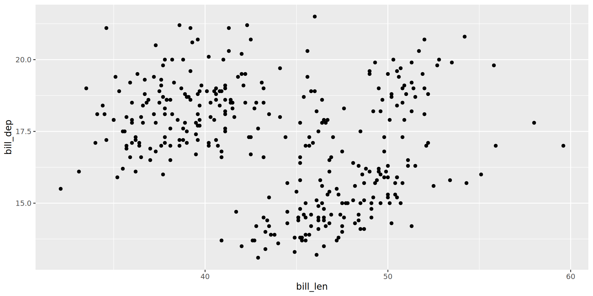
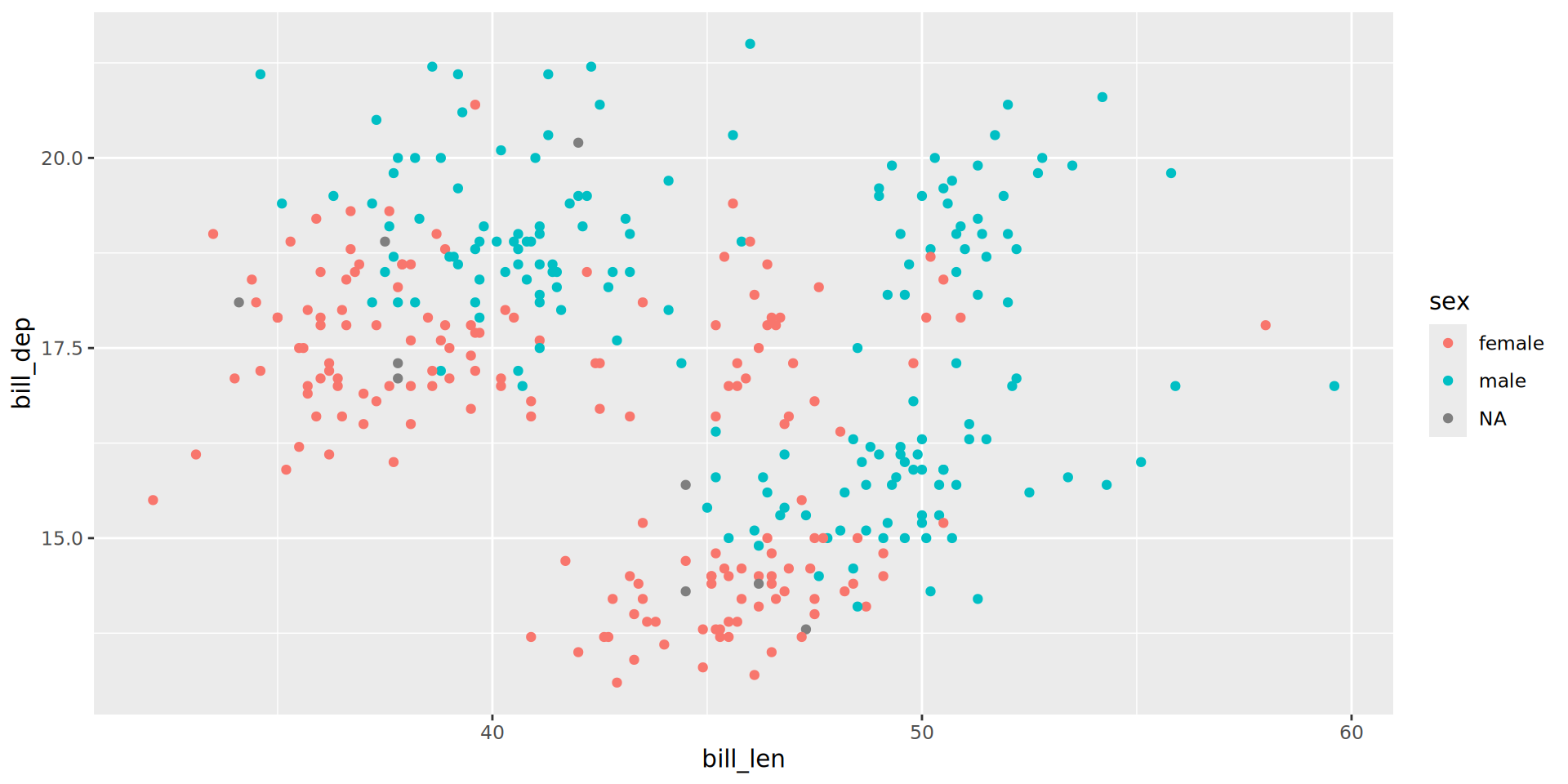
Using ggplot and mapping variables to colour, identify which of the categorical variables in penguins best explains the sub-grouping we observe in bill depth vs length.

Hints:

• glimpse() and summary() are useful functions for looking at your data.

• Even if you have found a variable that looks like it explains your data, did you check whether other variables also look like they explain the data?

Hypothesis: You cannot imagine a plot that can’t be made with ggplot

Challenge: I challenge you to clearly describe a plot or visualization that cannot be created in ggplot. There is a prize available.

Conditions:

• You must be able to describe this clearly, to the point where we as a group all agree on what you are requesting.

• This must be a plausible static visualization (i.e., no 3-dimensional, sound-producing scifi graph).

• You must give us your description by the start of Day 2 at the latest, and you must give us your description as soon as you come up with it.

• No LLMs.

• If, by the end of our final day, I haven’t been able to build OR find a plot that represents data as per your description, you win.

Summary

• Introduced R, the tidyverse dialect, and RStudio.

• Started a new project for easy file management.

• Learned to work in scripts for storing data.

• Introduced functions.

• Created new objects.

• Imported data.

• Looked at arguments, and default arguments.

• Introduced the pipe for clear and readable code.

• Covered errors and warnings.

• Introduced basic ggplot for exploratory analysis.