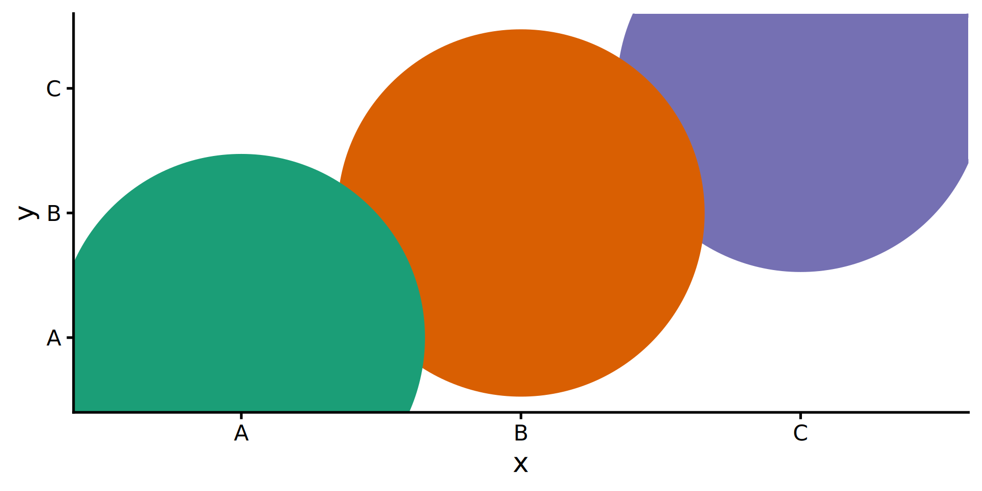
tibble(x = LETTERS[1:3],
y = x) |>
ggplot(aes(x, y)) +
geom_point(aes(colour = x),
show.legend = FALSE,
size = 125) +
scale_color_brewer(palette = "Dark2") +
theme_classic(20)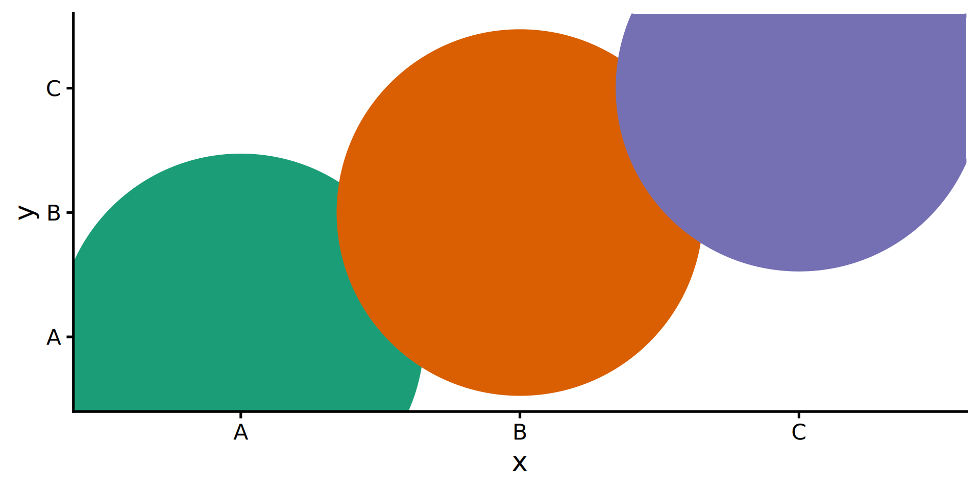
ggplot, part 3
Wednesday, 25 February 2026
ggbeeswarmlibrary(ggbeeswarm)
penguins |>
filter(!is.na(sex)) |>
ggplot(aes(y = body_mass_g,
x = species,
colour = sex)) +
geom_quasirandom(dodge.width = 1) #<<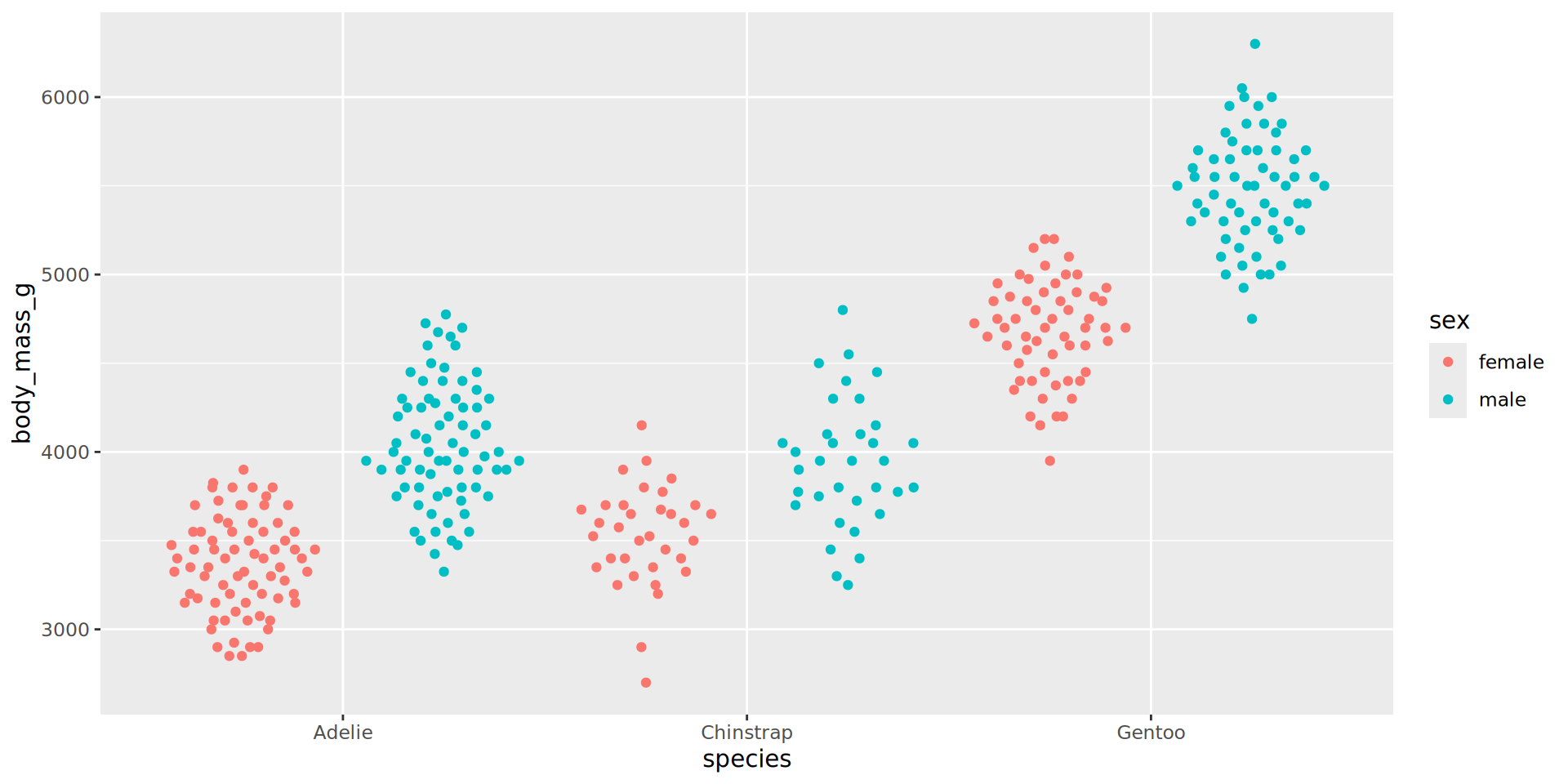
![]()
library(ggdist)
ggplot(penguins,
       aes(y = species,
           x = bill_depth_mm / bill_length_mm,
           color = species, fill = species)) +
  geom_violin(width = .5, fill = "white", alpha = 0.4,
              size = 1.1, trim = FALSE) +
  ggdist::stat_halfeye(
    adjust = .33, width = .67,
    alpha = 0.6, trim = FALSE,
    position = position_nudge(y = .35)) +
  ggbeeswarm::geom_quasirandom(groupOnX = FALSE,
                               alpha = .5, size = 3,
                               width = 0.25) +
  scale_color_brewer(palette = "Set1", type = "qual") +
  scale_fill_brewer(palette = "Set1", type = "qual") +
  labs(x = "Bill ratio", y = NULL) +
  theme(legend.position = "none",
        axis.line = element_blank(),
        panel.grid.major.x = element_line(colour = "grey90"),
        axis.ticks = element_blank())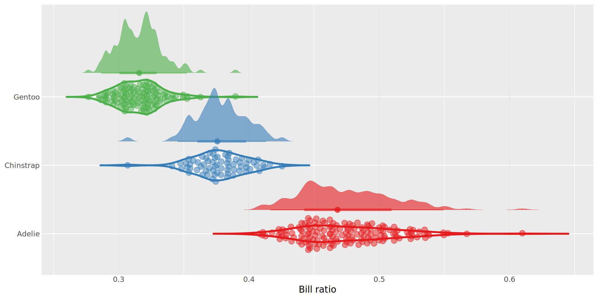
ggplot2 outputs dots as they appear in the input datatibble(x = LETTERS[1:3],
y = x) |>
ggplot(aes(x, y)) +
geom_point(aes(colour = x),
show.legend = FALSE,
size = 125) +
scale_color_brewer(palette = "Dark2") +
theme_classic(20)