scales::label_percent()(c(0.4, 0.6, .95))[1] "40%" "60%" "95%"scales::label_comma()(20^(1:4))[1] "20" "400" "8,000" "160,000"scales::breaks_log()(20^(1:3))[1] 10 30 100 300 1000 3000 10000ggplot, part 2
2026-02-25
Better: see Emil Hvitfeldt repo
scale_fill_hue()filter(starwars, !is.na(gender)) |>
ggplot(aes(y = gender,
fill = fct_lump_n(species, 8) |>
fct_infreq())) +
geom_bar(position = "fill") +
scale_fill_hue() +
labs(fill = "Top 8 Species\n(ranked)")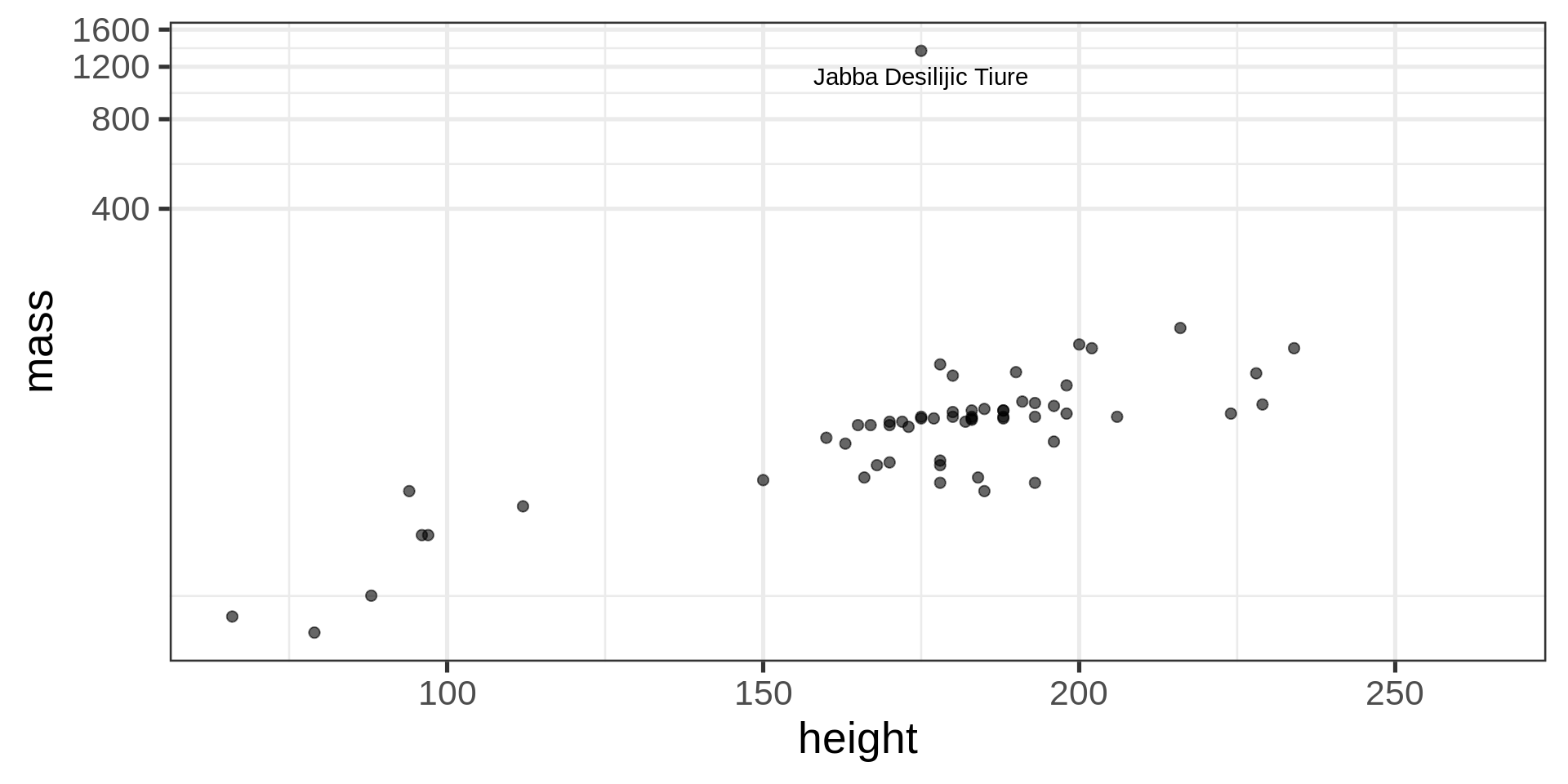
filter(starwars, !is.na(gender)) |>
ggplot(aes(y = gender,
          fill = fct_lump_n(species, 8) |>
                 fct_infreq())) +
  geom_bar(position = "fill") +
  scale_fill_brewer(palette = "Set1") +
  labs(fill = "Top 8 Species\n(ranked)")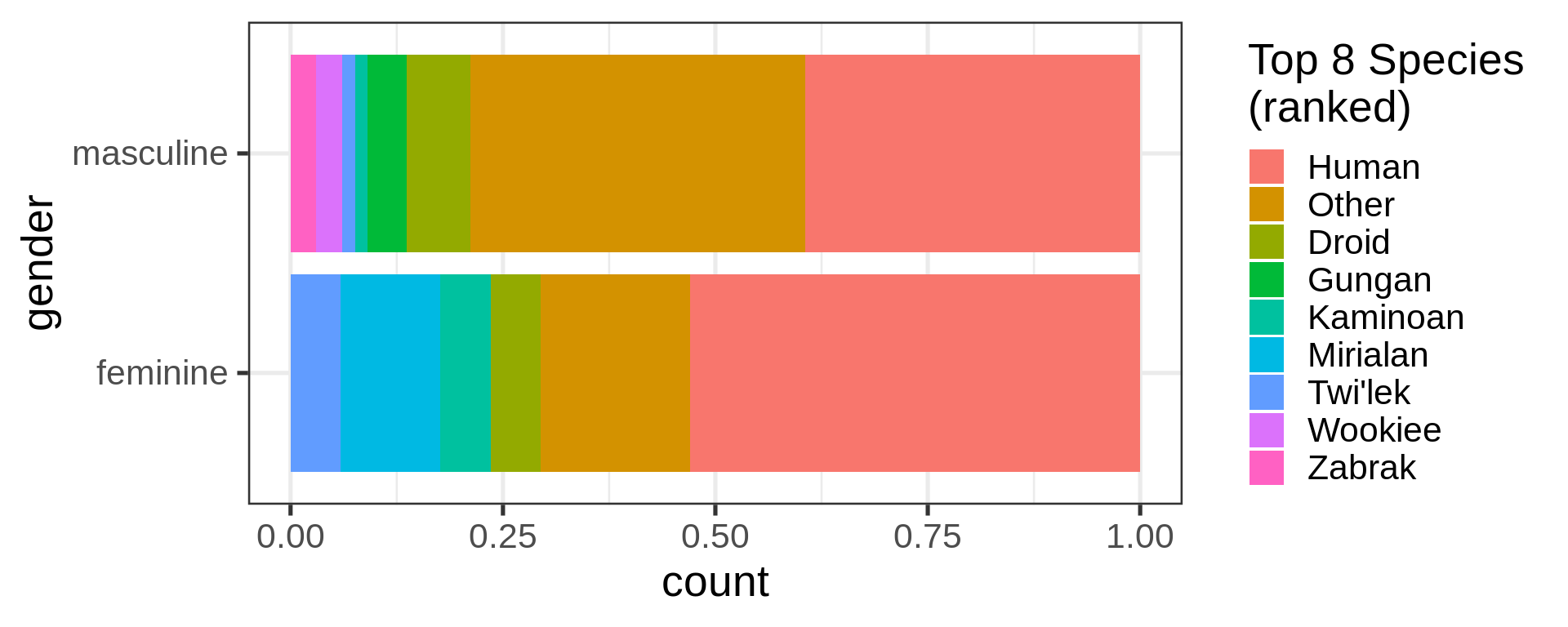
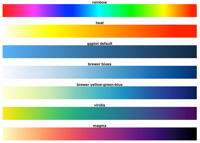
library(RColorBrewer)
par(mar = c(0, 4,
            0, 0))
display.brewer.all()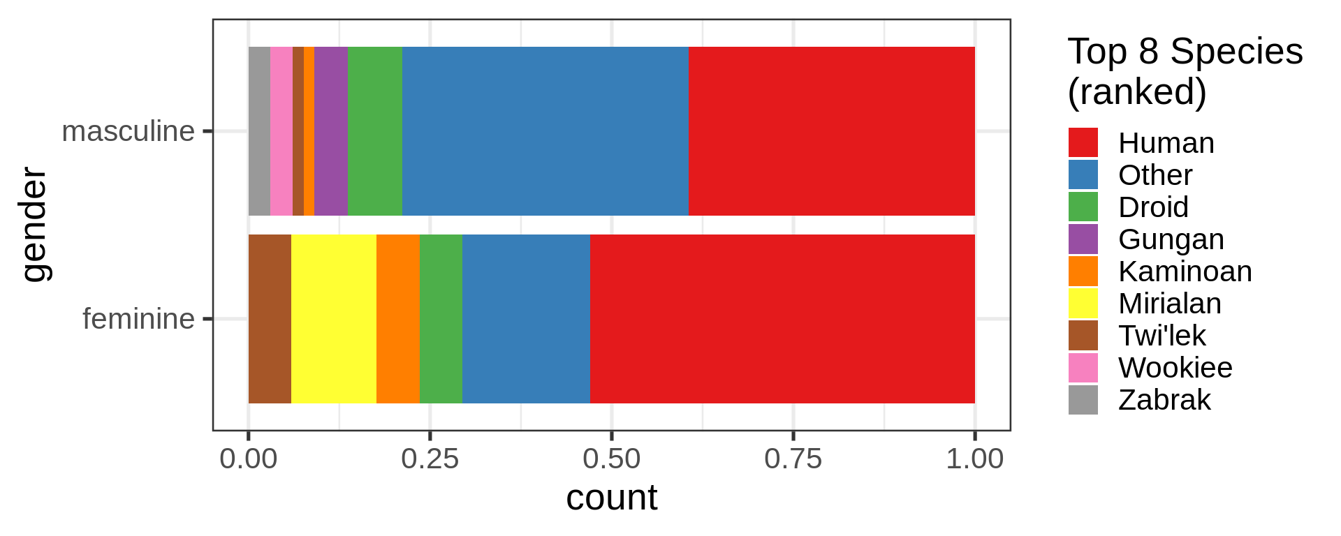
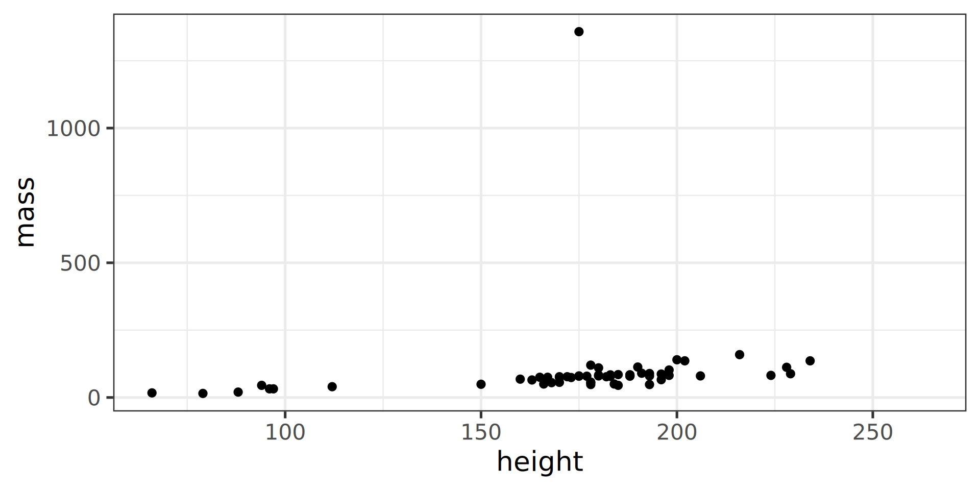
penguins |>
  ggplot(aes(x = bill_length_mm,
             y = bill_depth_mm,
             colour = body_mass_g)) +
  geom_point(alpha = 0.6, size = 5)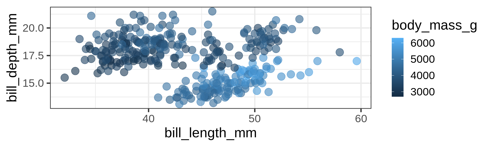
penguins |>
  ggplot(aes(x = bill_length_mm, y = bill_depth_mm,
             colour = body_mass_g)) +
  geom_point(alpha = 0.6, size = 5) +
  scale_color_viridis_c()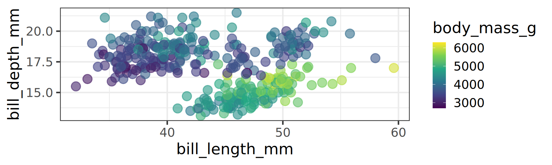
Viridis gradient is usually an improvement
Default ggplot2 is prints(!) well but on screens better off using viridis.
scale_color_viridis_c() c for continuous.
![]()
ggplot2 since v3.0 but no the default penguins |>
ggplot(aes(x = bill_length_mm, y = bill_depth_mm,
colour = species)) +
geom_point(alpha = 0.6, size = 5) +
scale_color_viridis_d()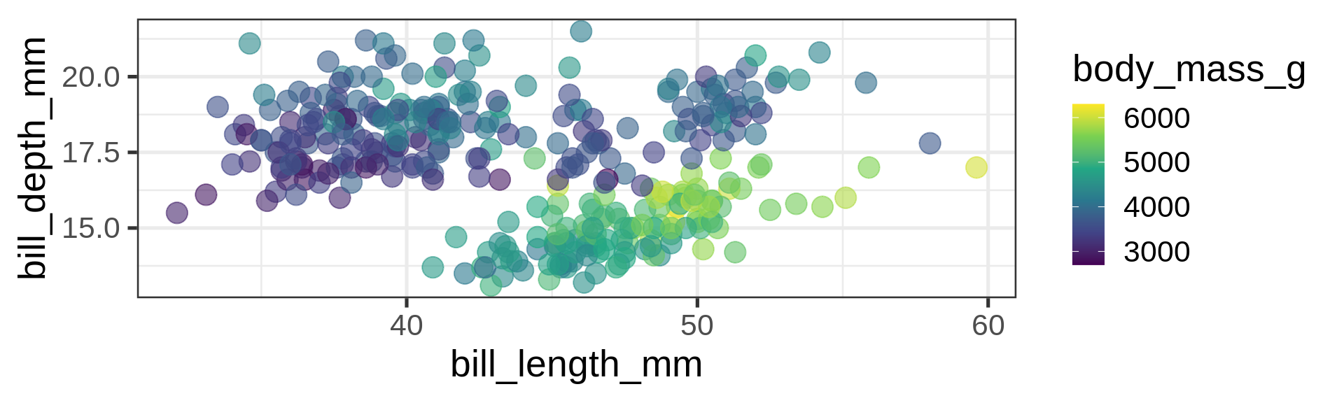
viridis optionpenguins |>
ggplot(aes(x = bill_length_mm, y = bill_depth_mm,
colour = body_mass_g)) +
geom_point(alpha = 0.6, size = 5) +
scale_color_binned(type = "viridis")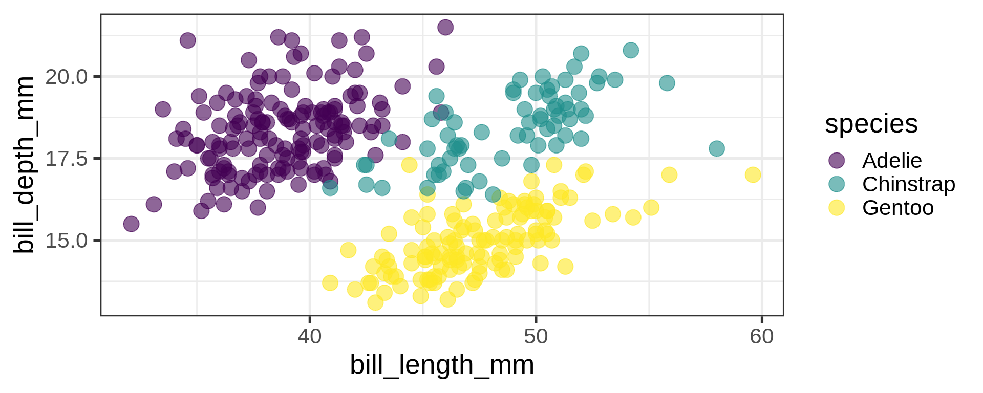
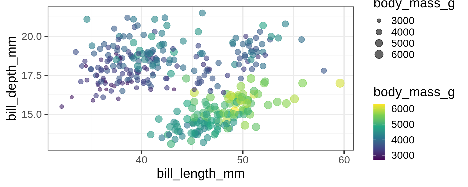
penguins |>
  ggplot(aes(x = bill_length_mm, y = bill_depth_mm,
             colour = body_mass_g,
             size = body_mass_g)) +
  geom_point(alpha = 0.6) +
  scale_color_viridis_c()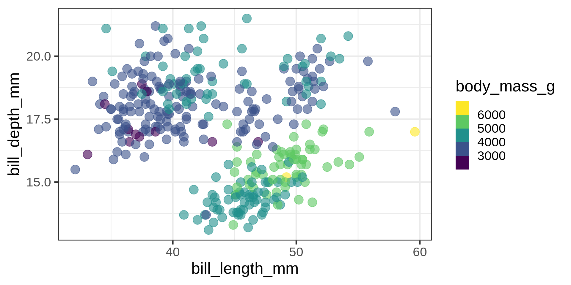
How to set the title
ggplot(penguins,
       aes(bill_depth_mm,
           bill_length_mm)) +
  geom_point()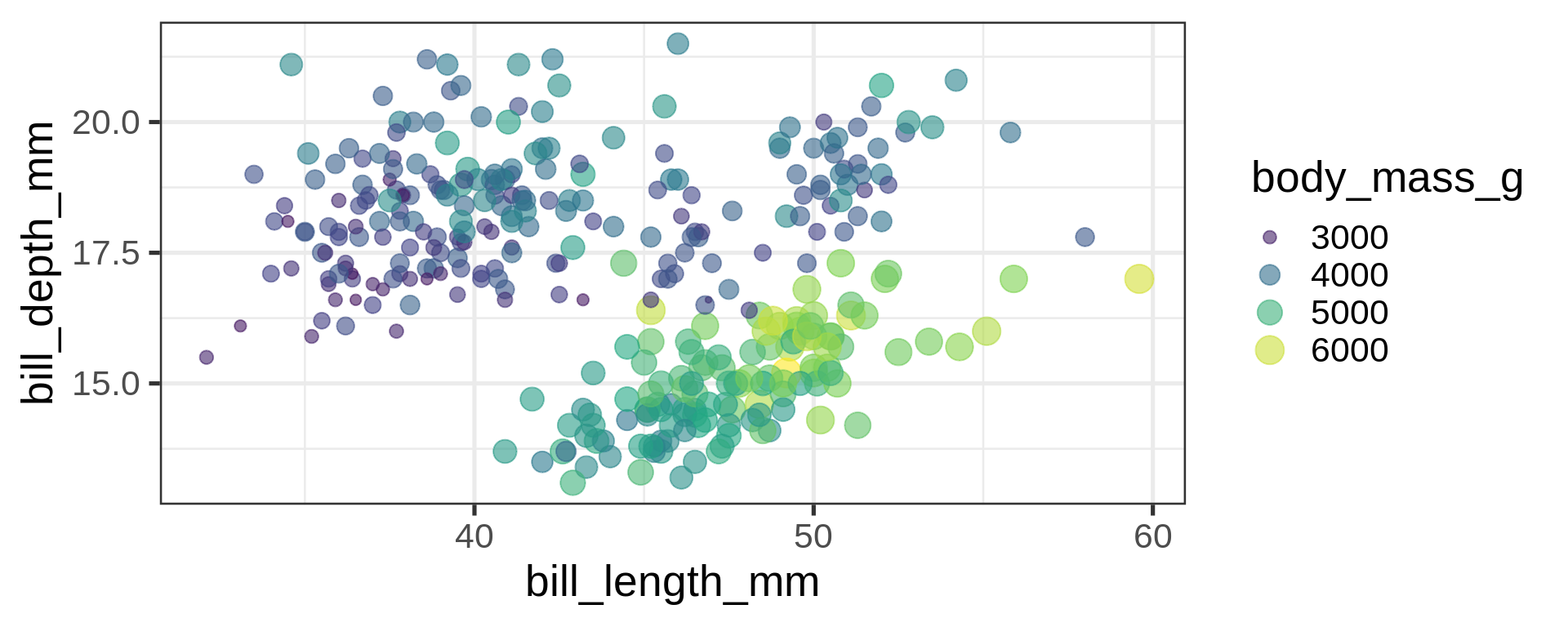
labs()ggplot(penguins, aes(bill_depth_mm, bill_length_mm)) +
geom_point() +
labs(x = "Bill depth (mm)",
y = "Bill length (mm)")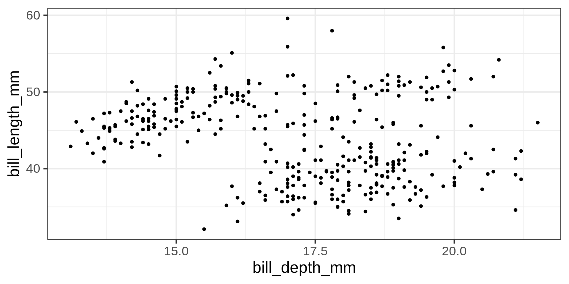
theme()ggplot(penguins, aes(bill_depth_mm, bill_length_mm)) + geom_point() +
labs(x = "Bill depth (mm)", y = "Bill length (mm)") +
theme(axis.title =
element_text(colour ="red"))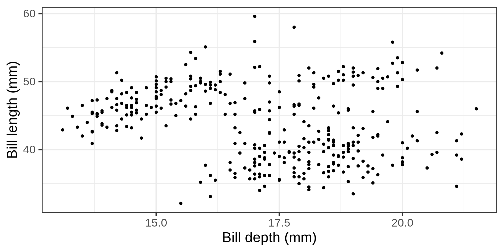
ggplot(penguins,
       aes(bill_depth_mm,
           bill_length_mm,
           colour = species)) +
  geom_point()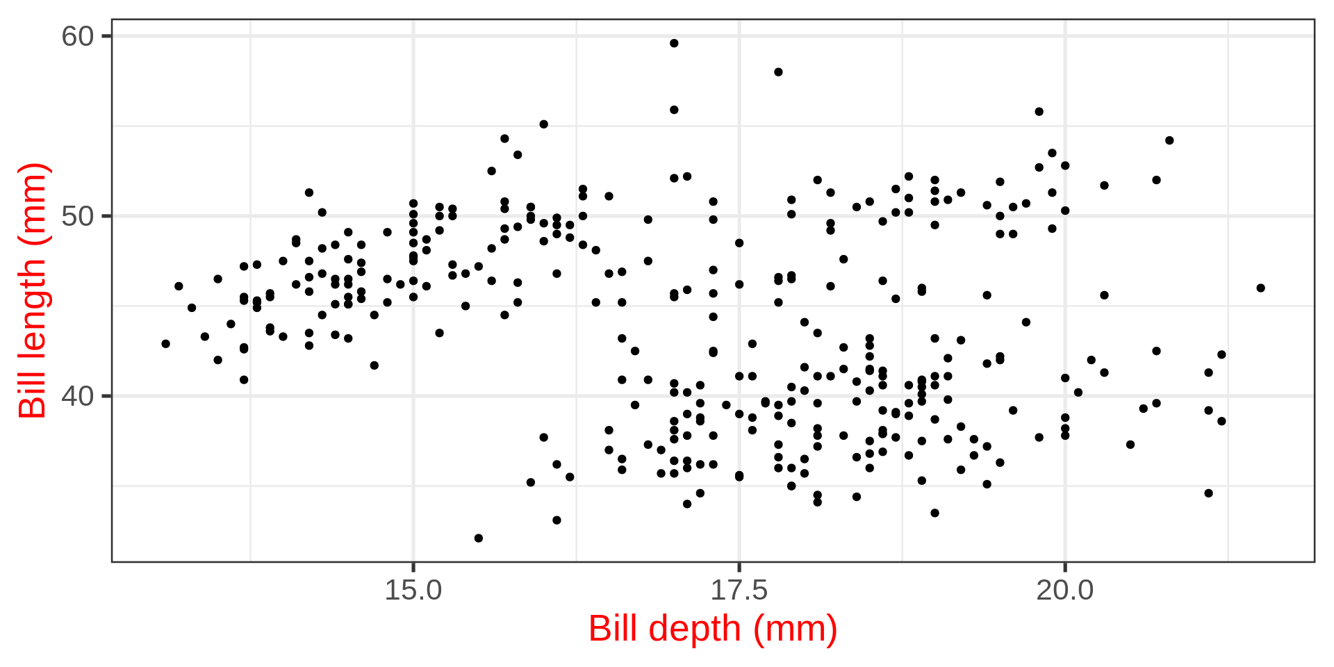
labs()ggplot(penguins, aes(bill_depth_mm, bill_length_mm, colour = species)) +
geom_point() +
labs(x = "Bill depth (mm)",
y = "Bill length (mm)",
colour = "Guide for\npenguins") 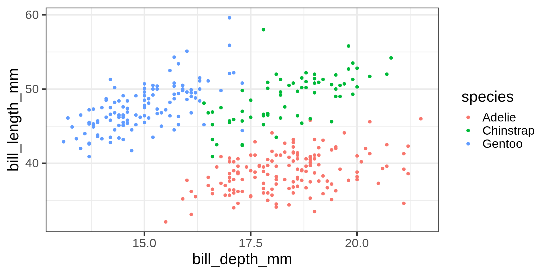
guides()ggplot(penguins, aes(bill_depth_mm, bill_length_mm, colour = species)) + geom_point() +
labs(x = "Bill depth (mm)", y = "Bill length (mm)") +
guides(colour =
guide_legend(title = "My penguin\nguide",
reverse = TRUE)) 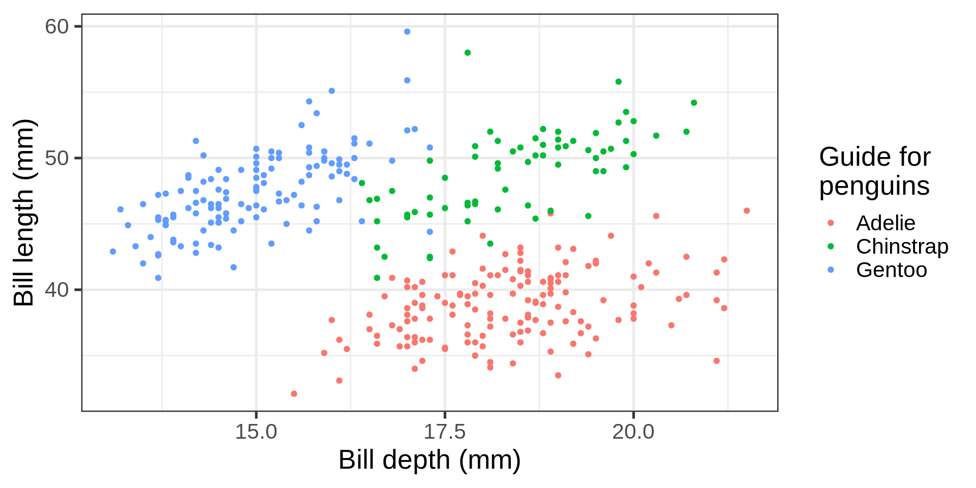
facet_wrap()facet_wrap()vars() function~)ggplot(penguins,
aes(bill_depth_mm,
bill_length_mm)) +
geom_point() +
facet_wrap(vars(species))
ncol = integernrow = integerfc <- ggplot(penguins,
aes(bill_depth_mm,
bill_length_mm)) +
geom_point()
fc + facet_wrap(vars(species), ncol = 2)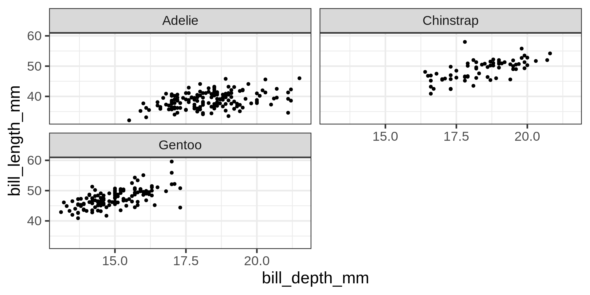
x or y (free_x / free_y)fc + facet_wrap(vars(species), scales = "free_y")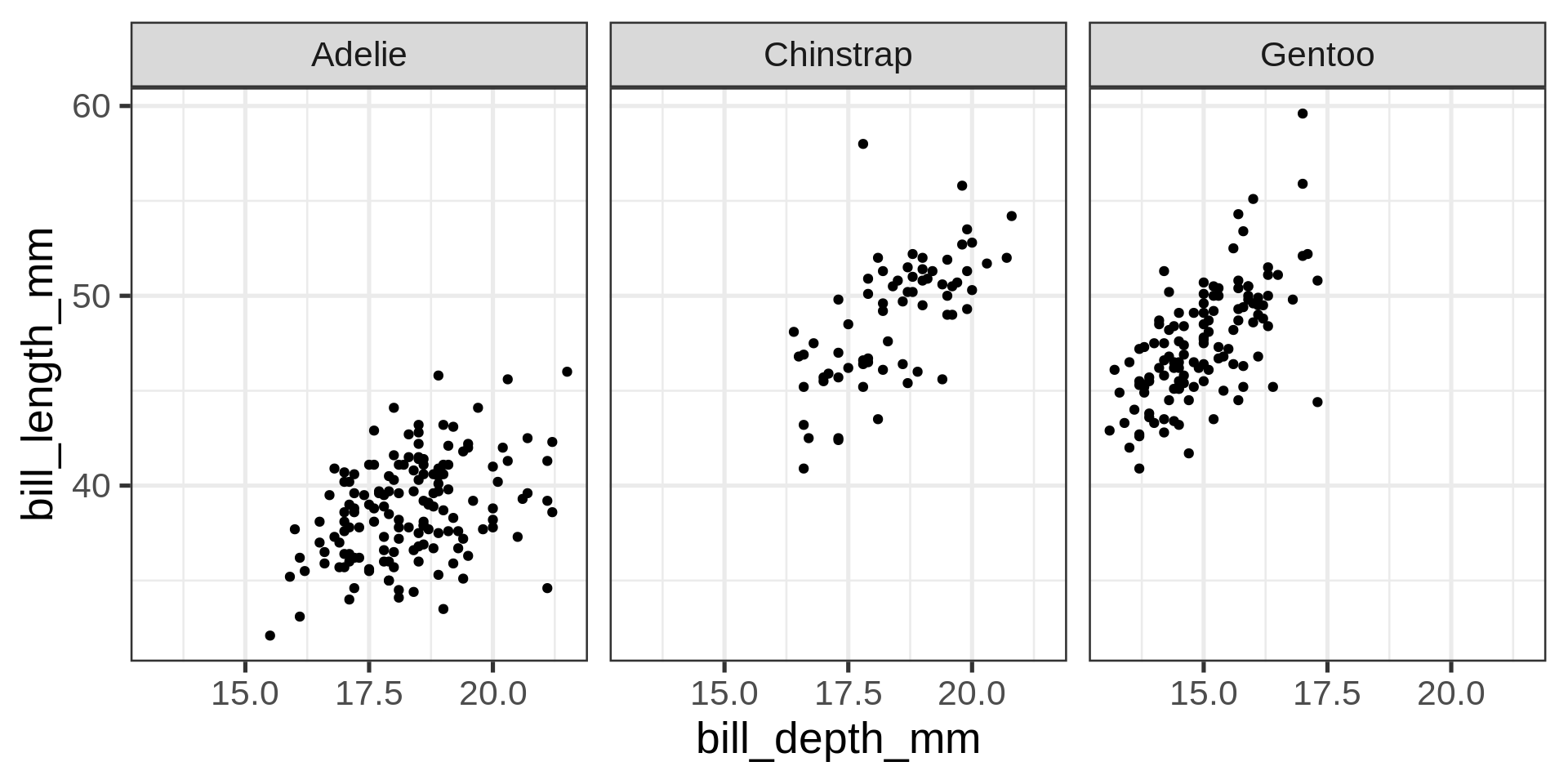
fc + facet_wrap(vars(species), scales = "free")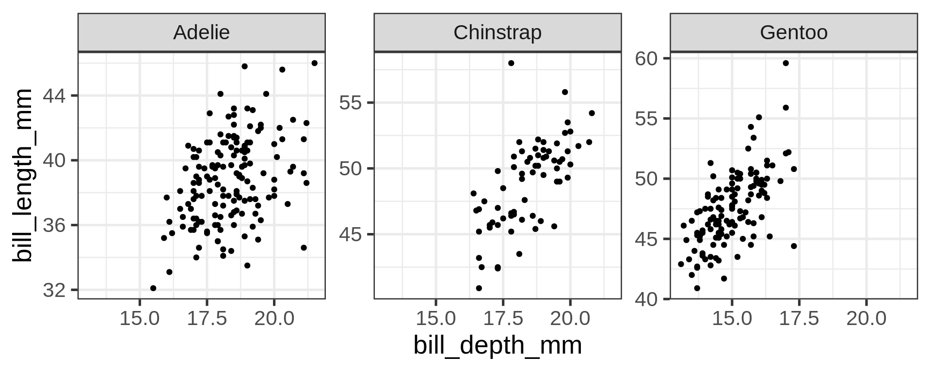
facet_grid() to lay out panels in a gridggplot(penguins,
aes(bill_depth_mm,
bill_length_mm)) +
geom_point() +
facet_grid(rows = vars(island), cols = vars(species))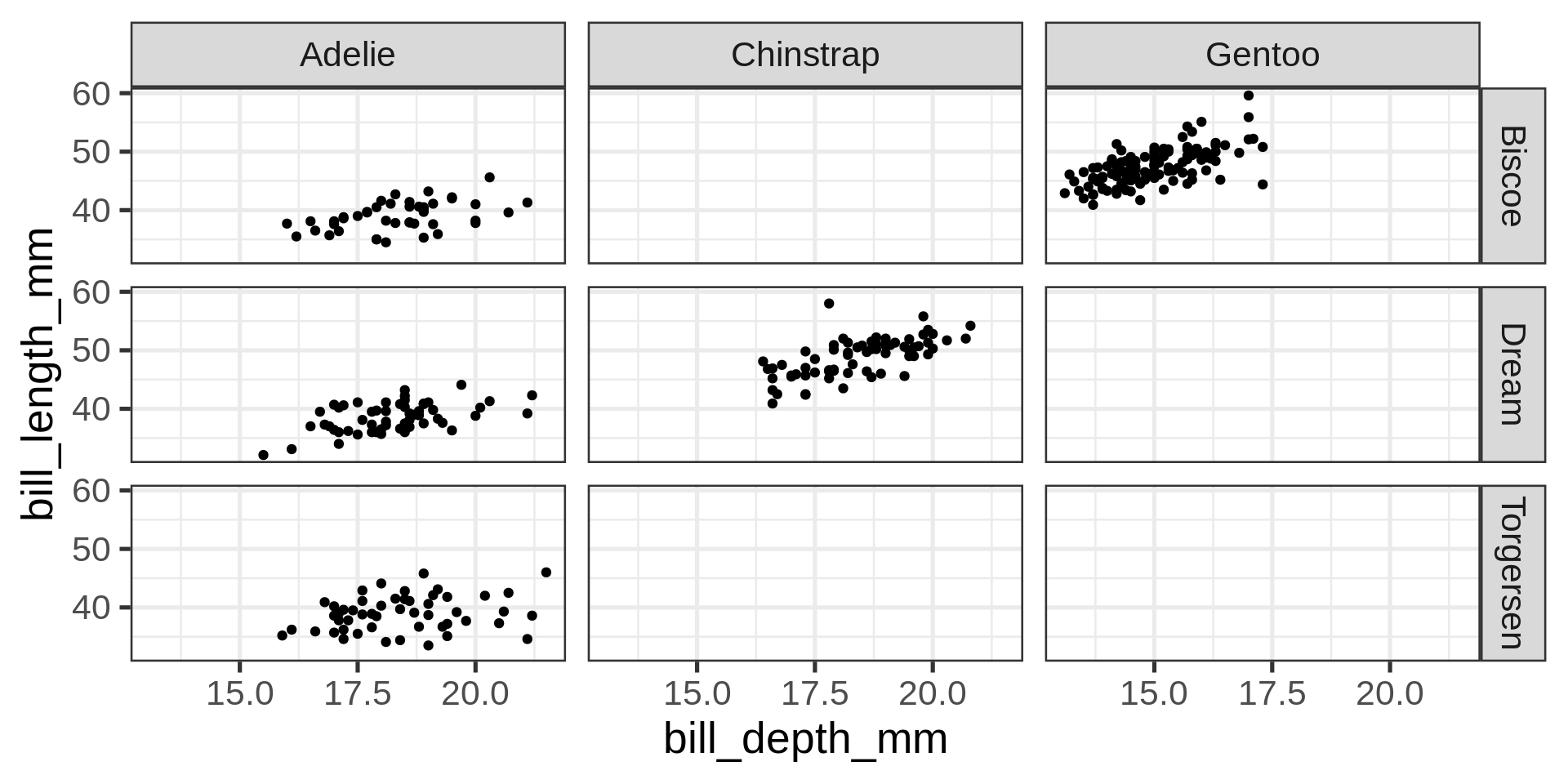
Grid lay out
~facet_grid() can also be used with one variable, complemented by a placeholder: .
ggplot(starwars) +
  geom_bar(aes(y = gender, fill = sex)) +
  facet_grid(fct_lump_min(species, 4) ~ .) +
  labs(y = NULL)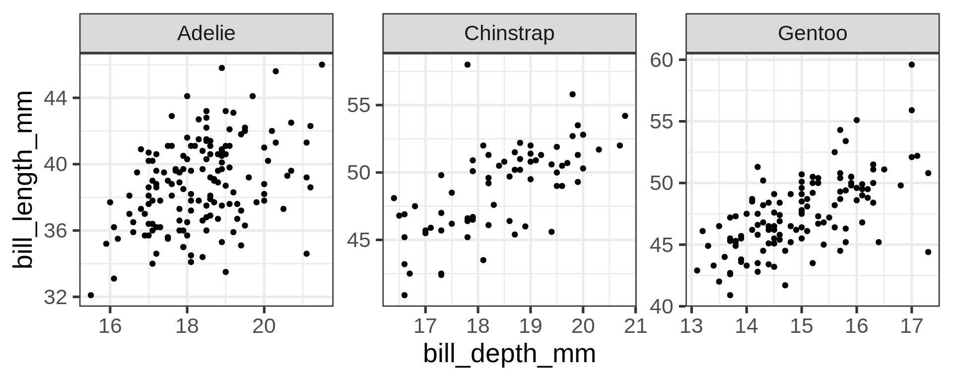
ggplot(starwars) +
  geom_bar(aes(y = gender, fill = sex)) +
  facet_grid(fct_lump_min(species, 4) ~ .,
             space = "free", scales = "free_y") +
  labs(y = NULL)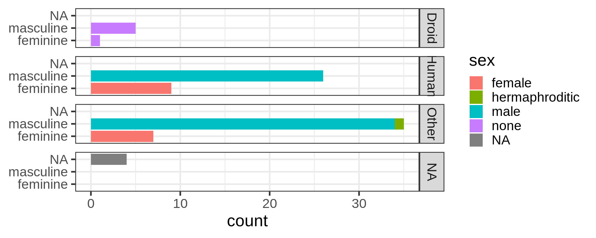
ggplot2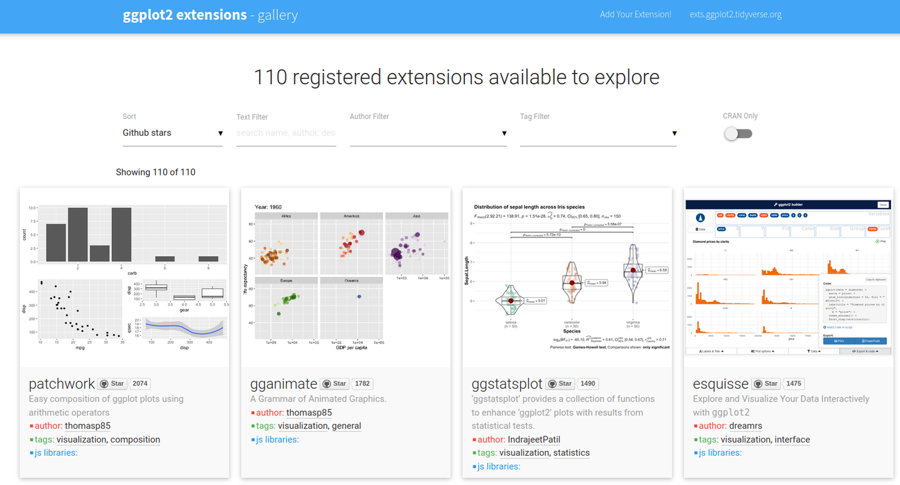
Finding working extensions
ggplot2 introduced the possibility for the community to create extensions, they are referenced on a dedicated site
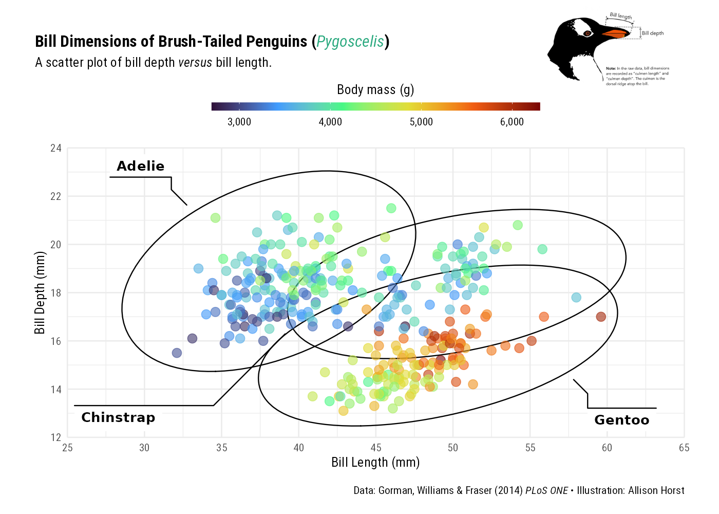
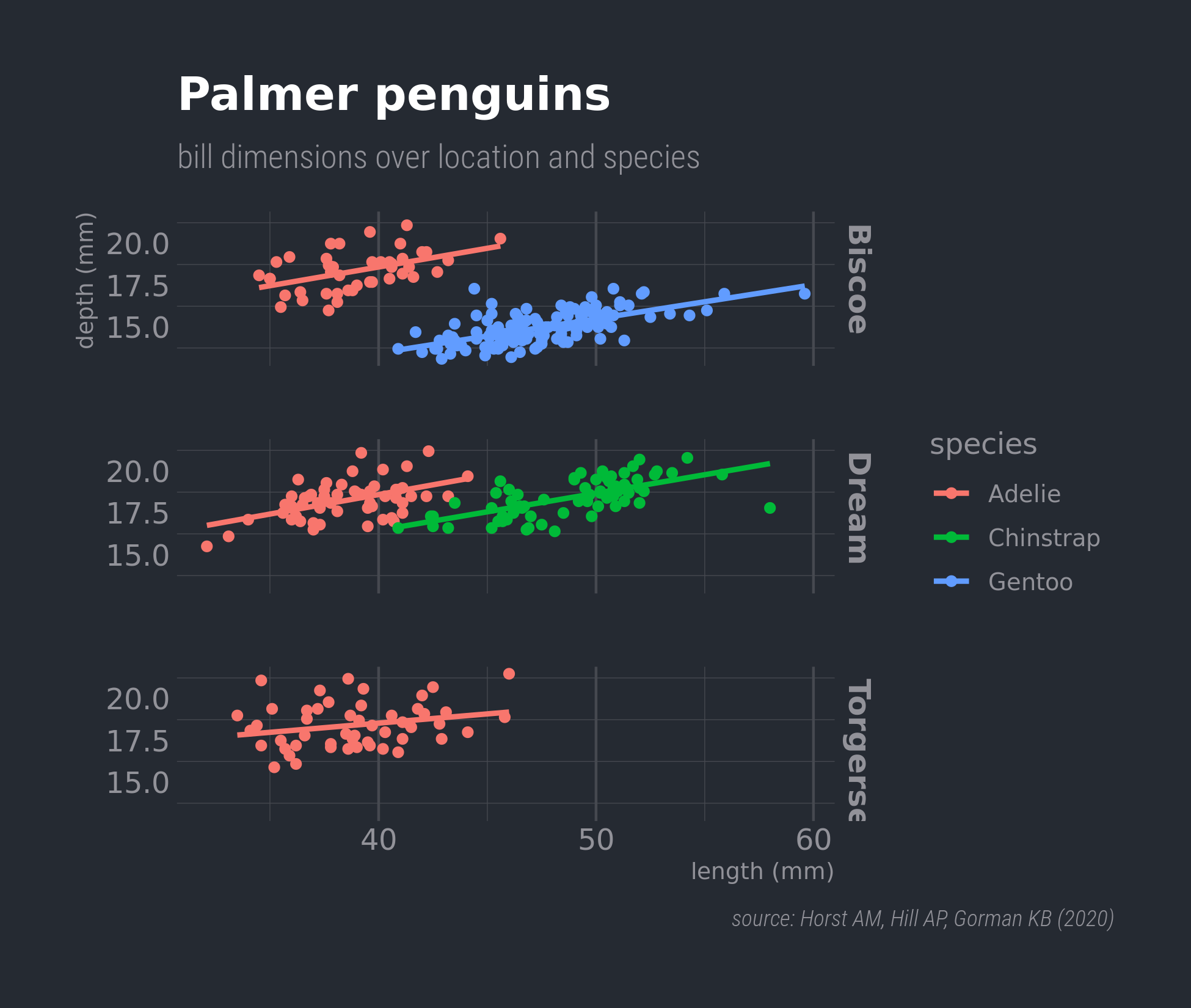
ggplot(penguins,
       aes(x = bill_length_mm,
           y = bill_depth_mm,
           colour = species)) +
  geom_point() +
  geom_smooth(method = "lm", formula = 'y ~ x',
      # no standard error ribbon
              se = FALSE) +
  facet_grid(island ~ .) +
  labs(x = "length (mm)", y = "depth (mm)",
       title = "Palmer penguins",
       subtitle = "bill dimensions over location and species",
       caption = "source: Horst AM, Hill AP, Gorman KB (2020)") +

  theme_dark(14) +
  # tweak the theme
  theme(panel.grid.major.y = element_blank(),
   panel.grid.major.x = element_line(size = 0.5),
   panel.background = element_rect(fill = "grey10"),
   plot.caption = element_text(face = "italic"),
   strip.text = element_text(face = "bold"),
   plot.caption.position = "plot")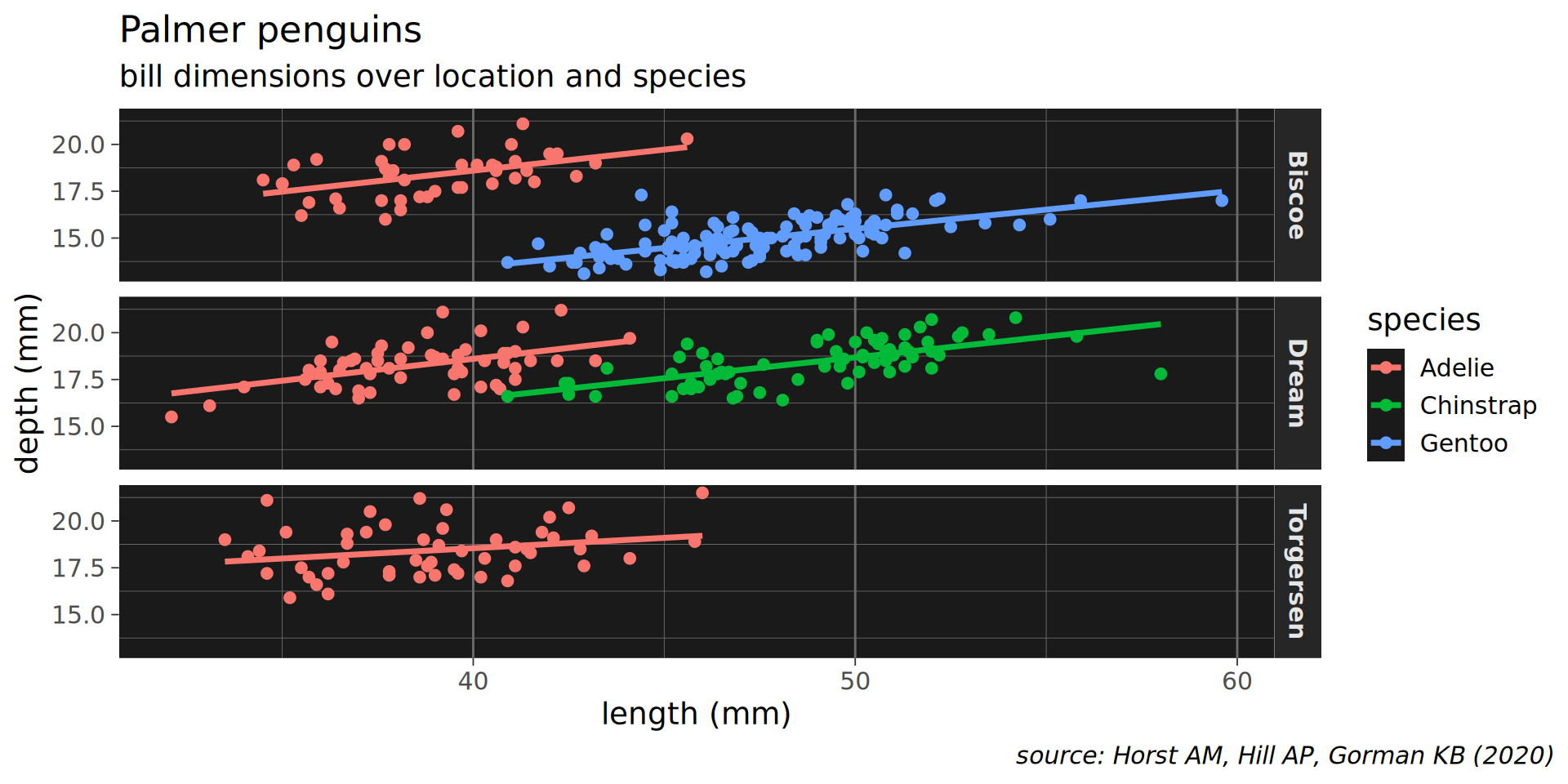
patchwork![]()
p1 <- ggplot(penguins,
aes(x = species)) +
geom_bar() +
labs(title = "Species distribution")
p2 <- ggplot(penguins,
aes(y = island)) +
geom_bar() +
labs(title = "Island but flipped")
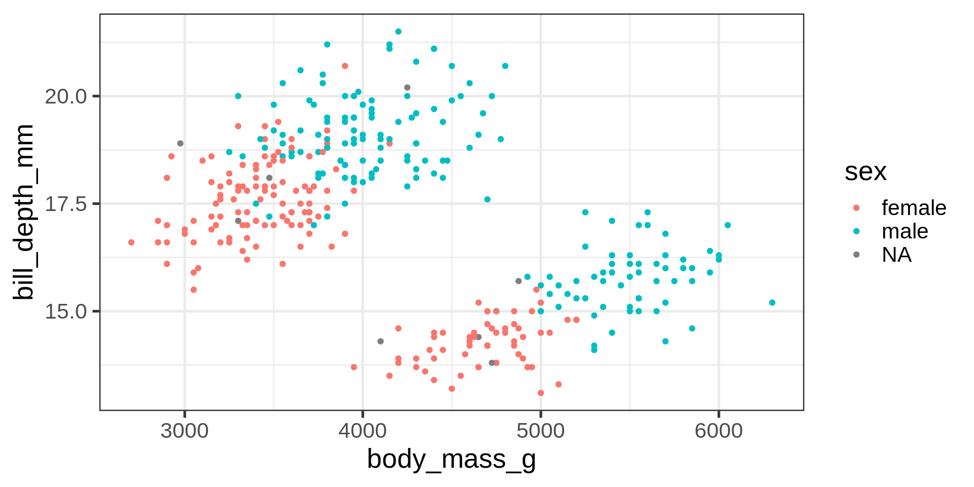
p3 <- ggplot(penguins,
aes(x = body_mass_g,
y = bill_depth_mm,
colour = sex)) +
geom_point()p1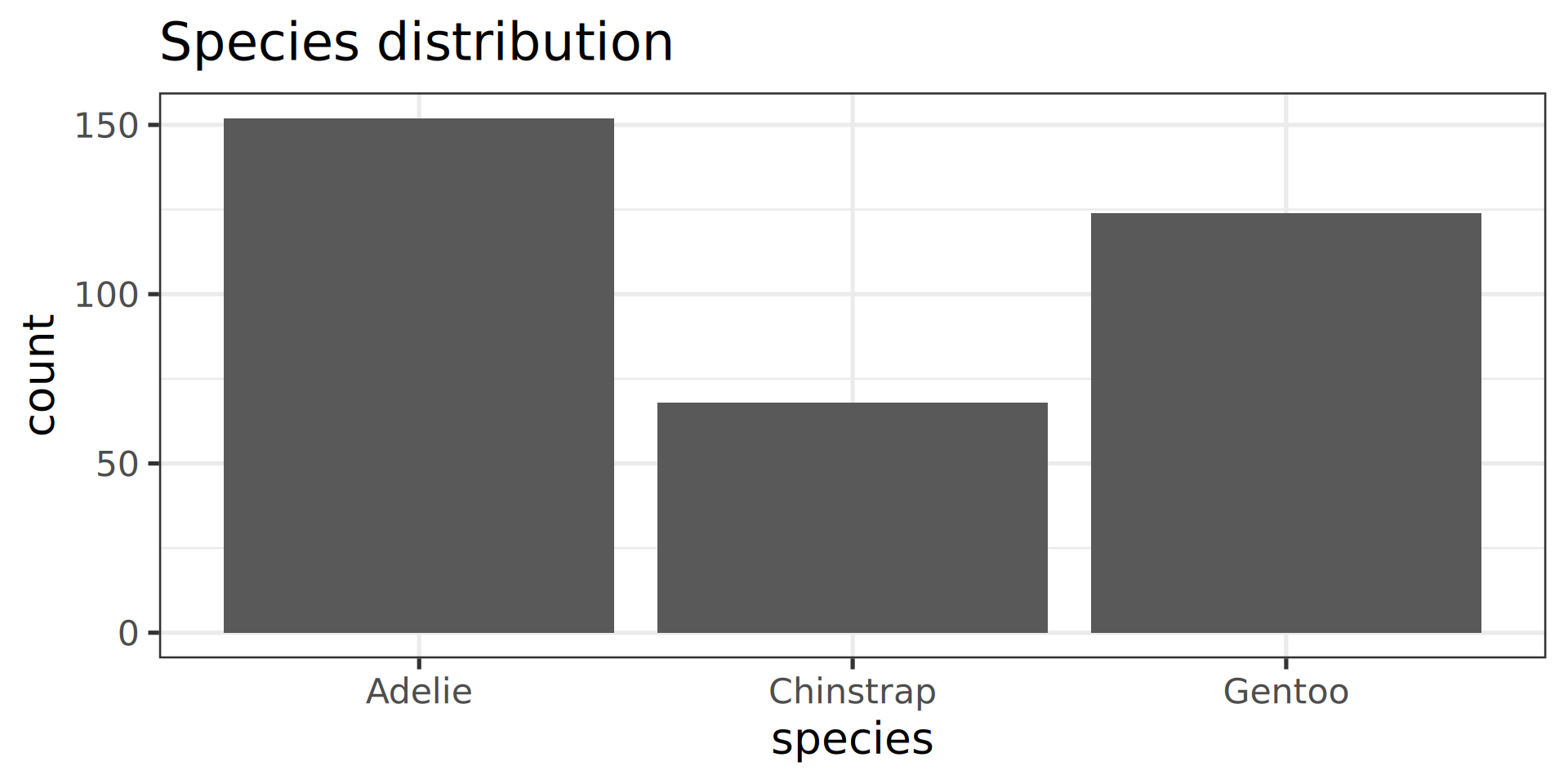
p2
Now, compose them!
p3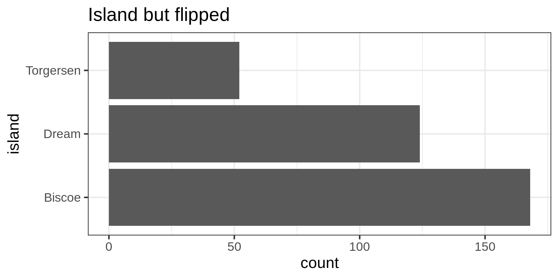
patchwork![]()
library(patchwork)
(( p1 | p2 ) / p3) +
  # add tags and main title
  plot_annotation(tag_levels = 'A',
                  title = 'Plots about penguins') &
  # modify all plots recursively
  theme_minimal() +
  theme(text = element_text('Roboto'))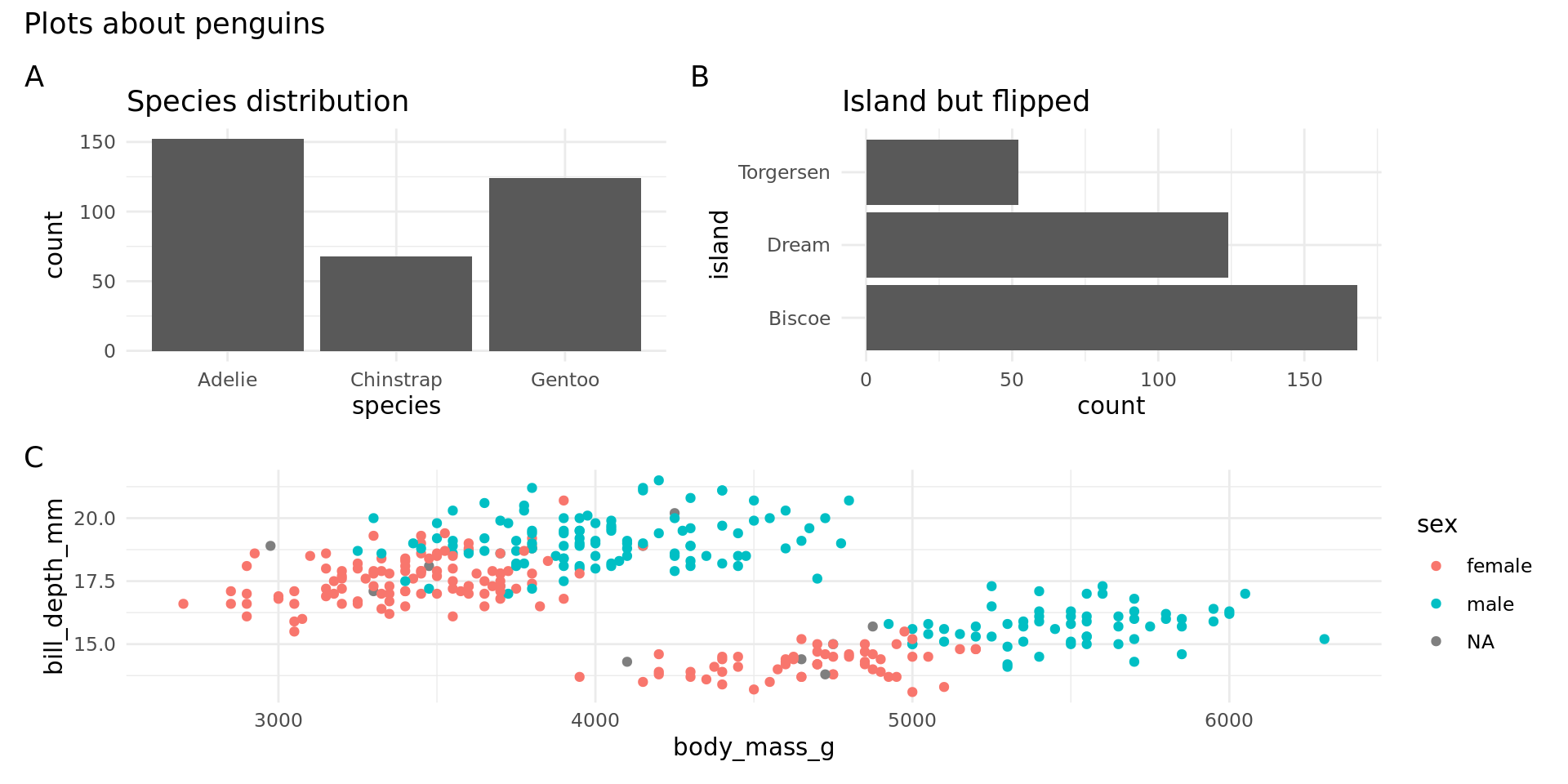
![]()
library(geomtextpath)
ggplot(penguins,
       aes(x = bill_length_mm, y = bill_depth_mm, colour = species)) +
  geom_point(alpha = 0.3) +
  stat_ellipse(aes(label = species),
    geom = "textpath", hjust = c(0.55)) +
  theme_bw(14) + guides(color = "none")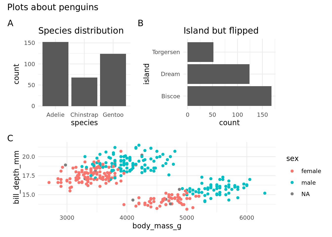
ggplot(penguins,
       aes(x = bill_length_mm / bill_depth_mm,
           colour = species)) +
  stat_density(aes(label = species),
    geom = "textpath", hjust = c(0.25)) +
  theme_bw(14) + guides(color = "none")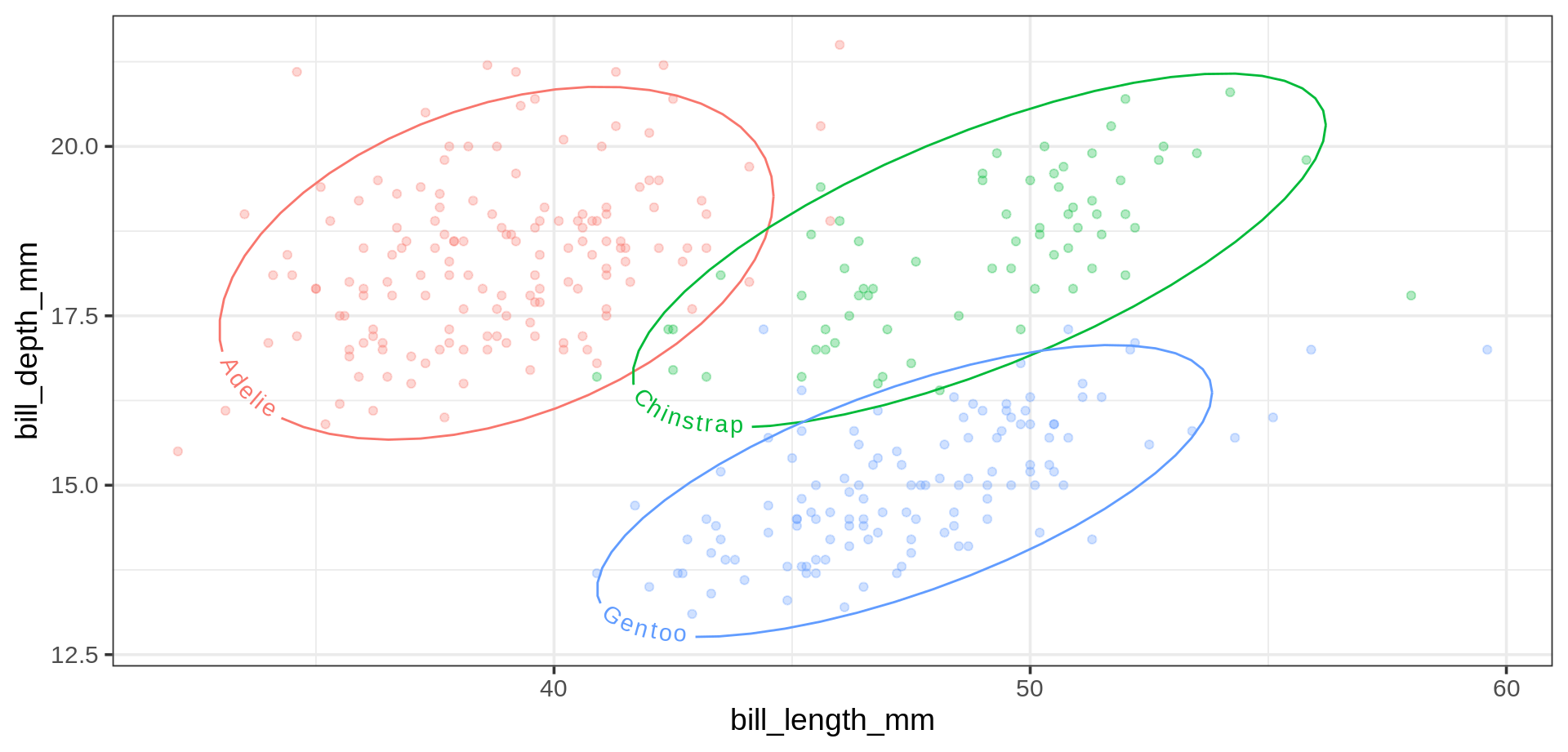
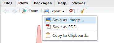
ggplot object, 2nd argument, here p or last_plot()svg, png, svg, etc.)ggsave("my_name.png", p, width = 60, height = 30, units = "mm")
ggsave("my_name.pdf", last_plot(), width = 50, height = 50, units = "mm")fig-height, fig-widthfig-asp…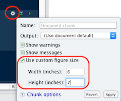
esquisse Rstudio addin by dreamRs![]()