library(ggplot2)
swiss |>
  ggplot() +
  aes(x = Education,
      y = Examination) +
  geom_point() +
scale_colour_brewer()Plotting data
ggplot, part 1
2026-02-25
Introduction
Elements of ggplot2
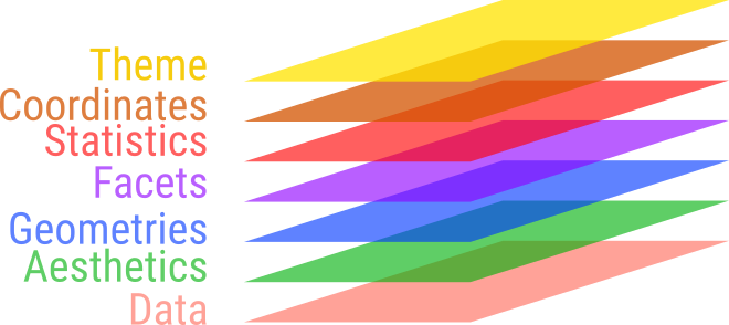
Graphs are split into parts
- Separate axis, curve(s), labels.
- 3 elements are typically found
- data,
- mapping as aesthetics,
- layers of geometries or statistics.
Result
What if we want to split into panels for circles and squares?
Faceting
Split by shape, aka trellis or lattice plots
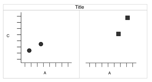
Redundancy
- shape and facets provide the same information.
- The
shapeaesthetic is free for another variable.
Combining parts
All ggplot elements are functions
Using the pipe out of habit
  ggplot(swiss) |>
  aes(x = Education,
      y = Examination) |>
  geom_point() +
  scale_colour_brewer()
Error:
! Cannot add <ggproto> objects together.
ℹ Did you forget to add this object to a <ggplot> object?Capabilities in ggplot - data
ggplot(data = penguins)
Capabilities in ggplot - mapping
ggplot(data = penguins) +
  aes(x = flipper_len,
      y = body_mass)
Capabilities in ggplot - geometric layer
ggplot(data = penguins) +
  aes(x = flipper_len,
      y = body_mass) +
geom_point(alpha = 0.5) 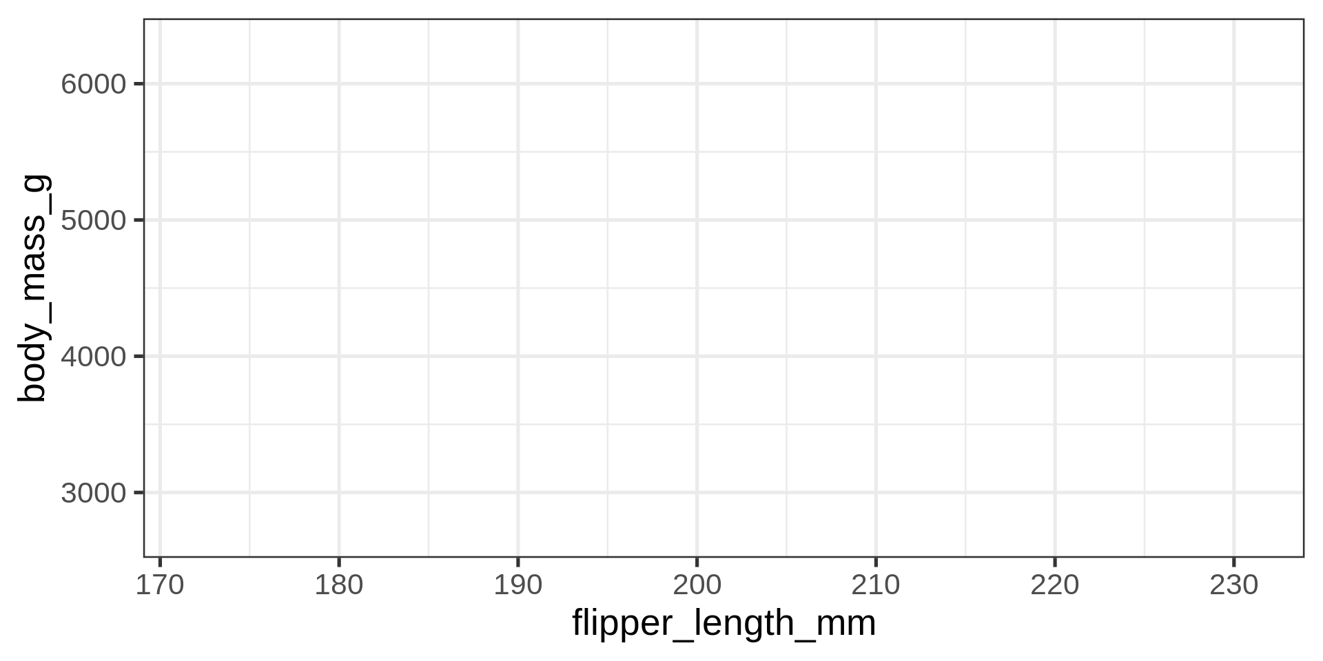
Single, unmapped parameter applied to all points
Capabilities in ggplot - geometric layer
ggplot(data = penguins) +
  aes(x = flipper_len,
      y = body_mass) +
  geom_point(aes(color = sex),
alpha = 0.5) 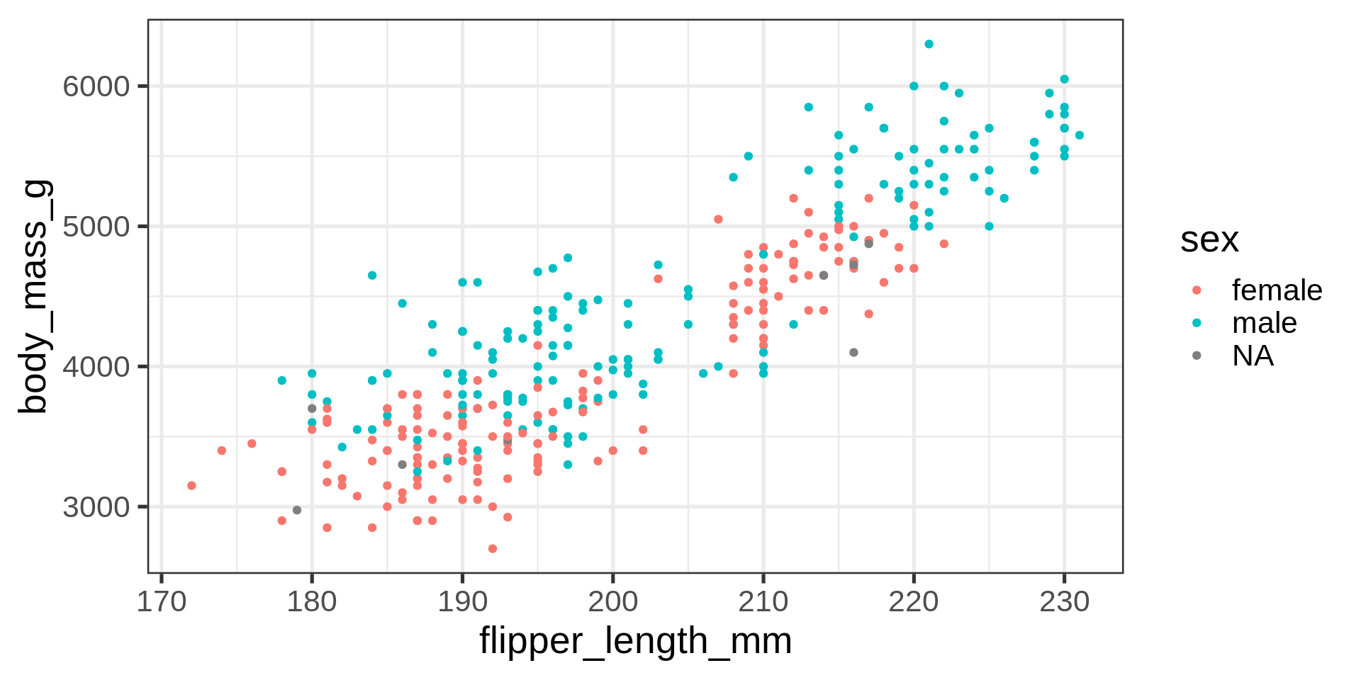
Overplotting
Frequent issue with scatter plots - too much empty space and not enough resolution where needed
Capabilities in ggplot - statistics layer
(ggplot(data = penguins) +
  aes(x = flipper_len,
      y = body_mass) +
  geom_point(aes(color = sex)) +
  stat_density_2d()
     -> gg_peng)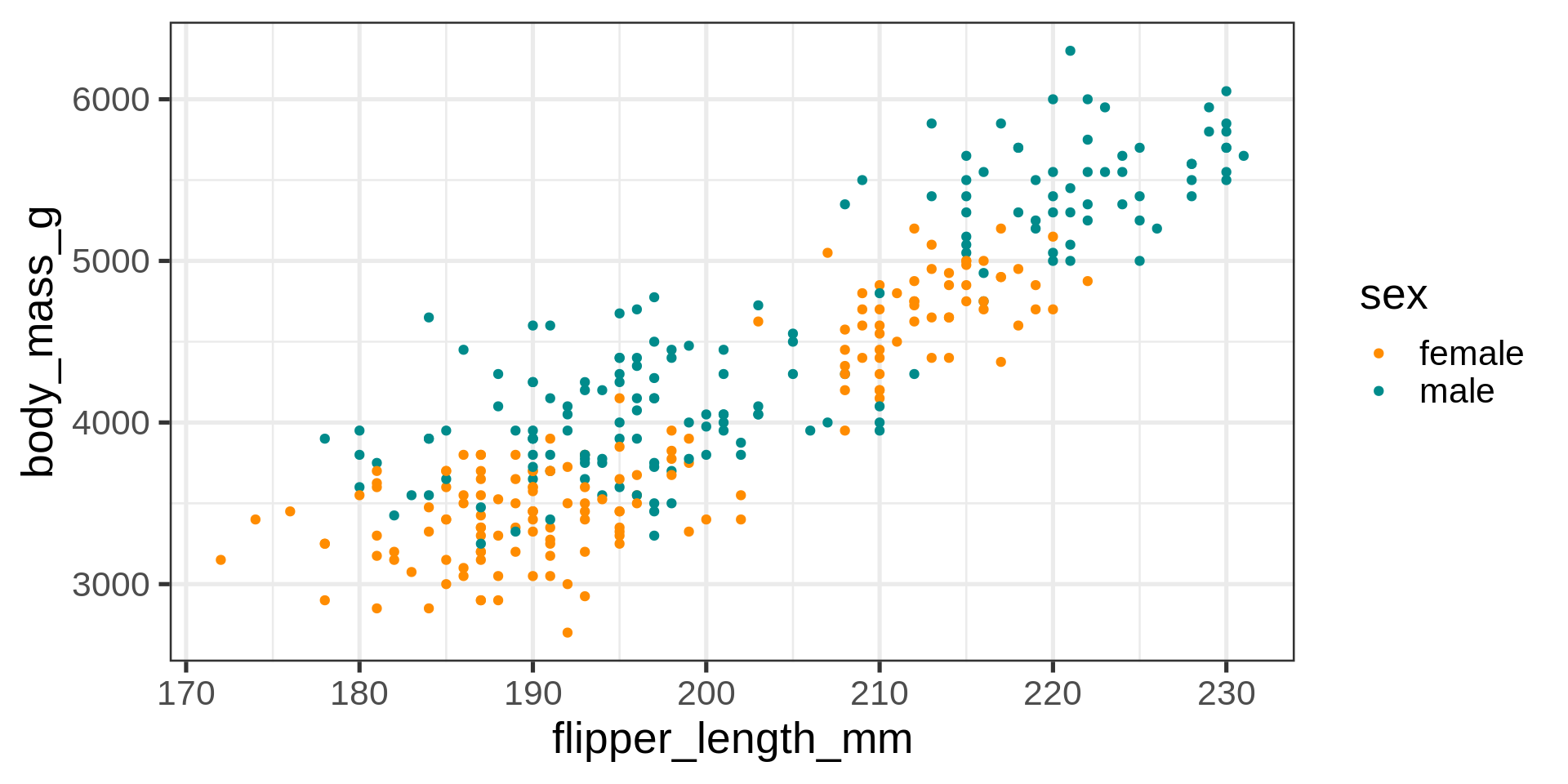
Capabilities in ggplot - layers reordered
(ggplot(data = penguins) +
  aes(x = flipper_len,
      y = body_mass) +
  stat_density_2d() +
  geom_point(aes(color = sex))
     -> gg_peng)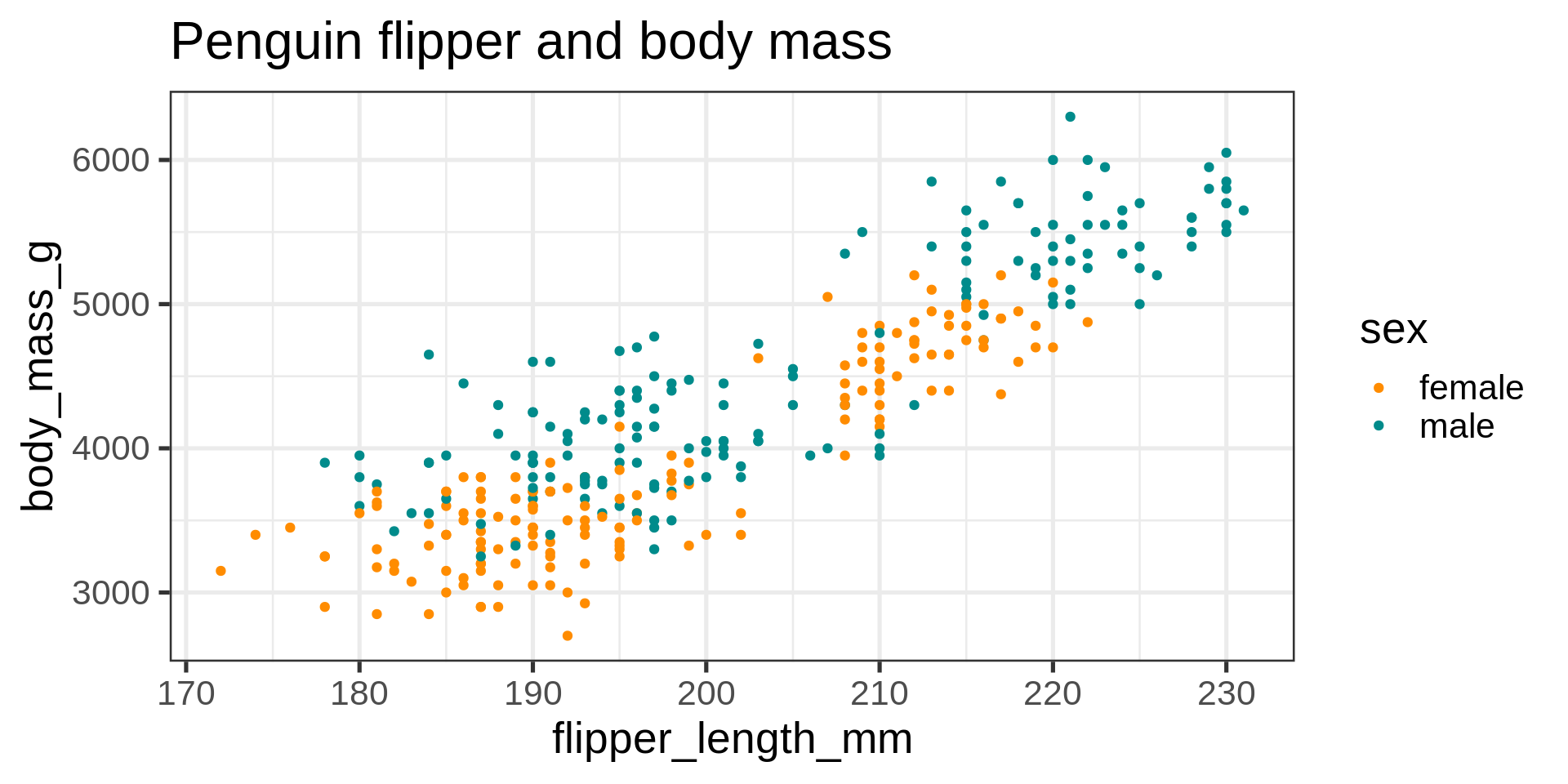
Capabilities in ggplot - labels
gg_peng +
  labs(title = "Penguin flipper and body mass")
Capabilities in ggplot
gg_peng +
  labs(title = "Penguin flipper and body mass",
       x = "Flipper length (mm)",
       y = "Body mass (g)")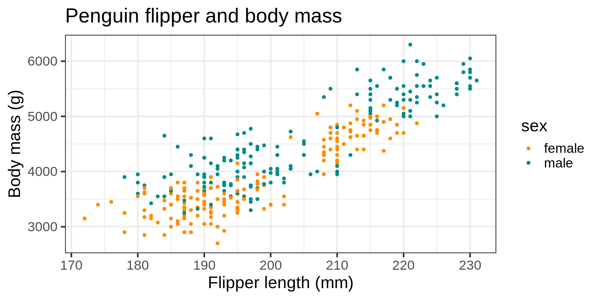
Capabilities in ggplot
gg_peng +
  labs(title = "Penguin flipper and body mass",
       x = "Flipper length (mm)",
       y = "Body mass (g)")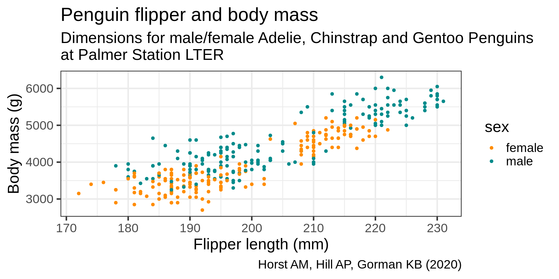
description <- "Dimensions for male/female Adelie, Chinstrap and Gentoo Penguins\nat Palmer Station LTER"Capabilities in ggplot
gg_peng +
  labs(title = "Penguin flipper and body mass",
       caption = "Horst AM, Hill AP, Gorman KB (2020)",
       subtitle = description,
       x = "Flipper length (mm)",
       y = "Body mass (g)")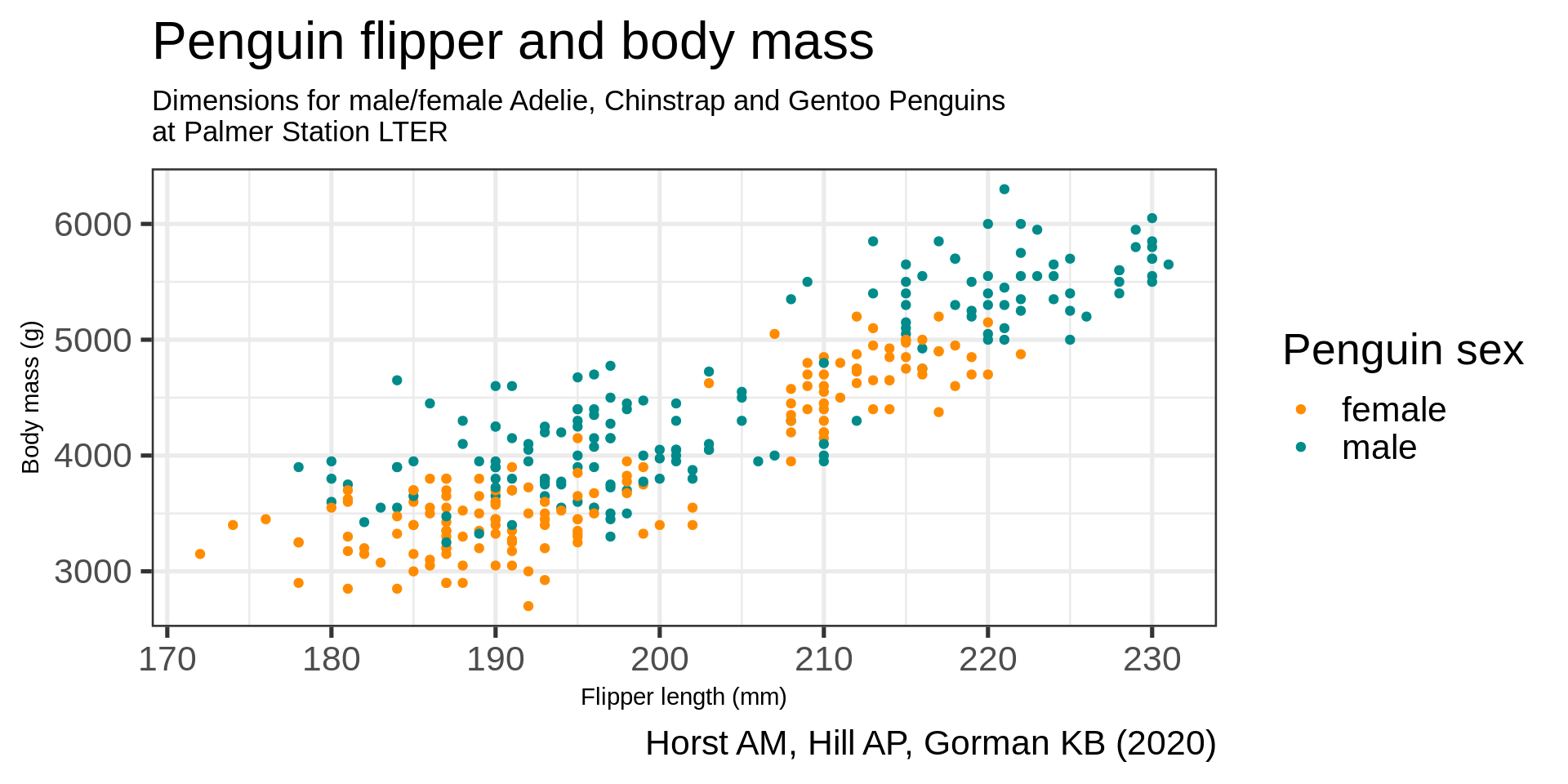
Capabilities in ggplot
gg_peng +
  labs(title = "Penguin flipper and body mass",
       caption = "Horst AM, Hill AP, Gorman KB (2020)",
       subtitle = description,
       x = "Flipper length (mm)",
       y = "Body mass (g)",
       color = "Penguin sex") -> gg_peng_labs

gg_peng_labs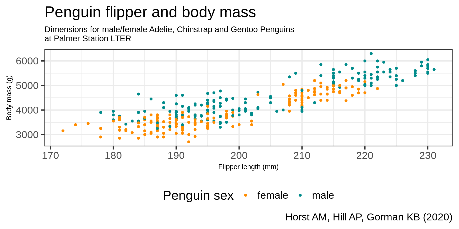
Capabilities in ggplot - theme
gg_peng_labs +
theme_bw() 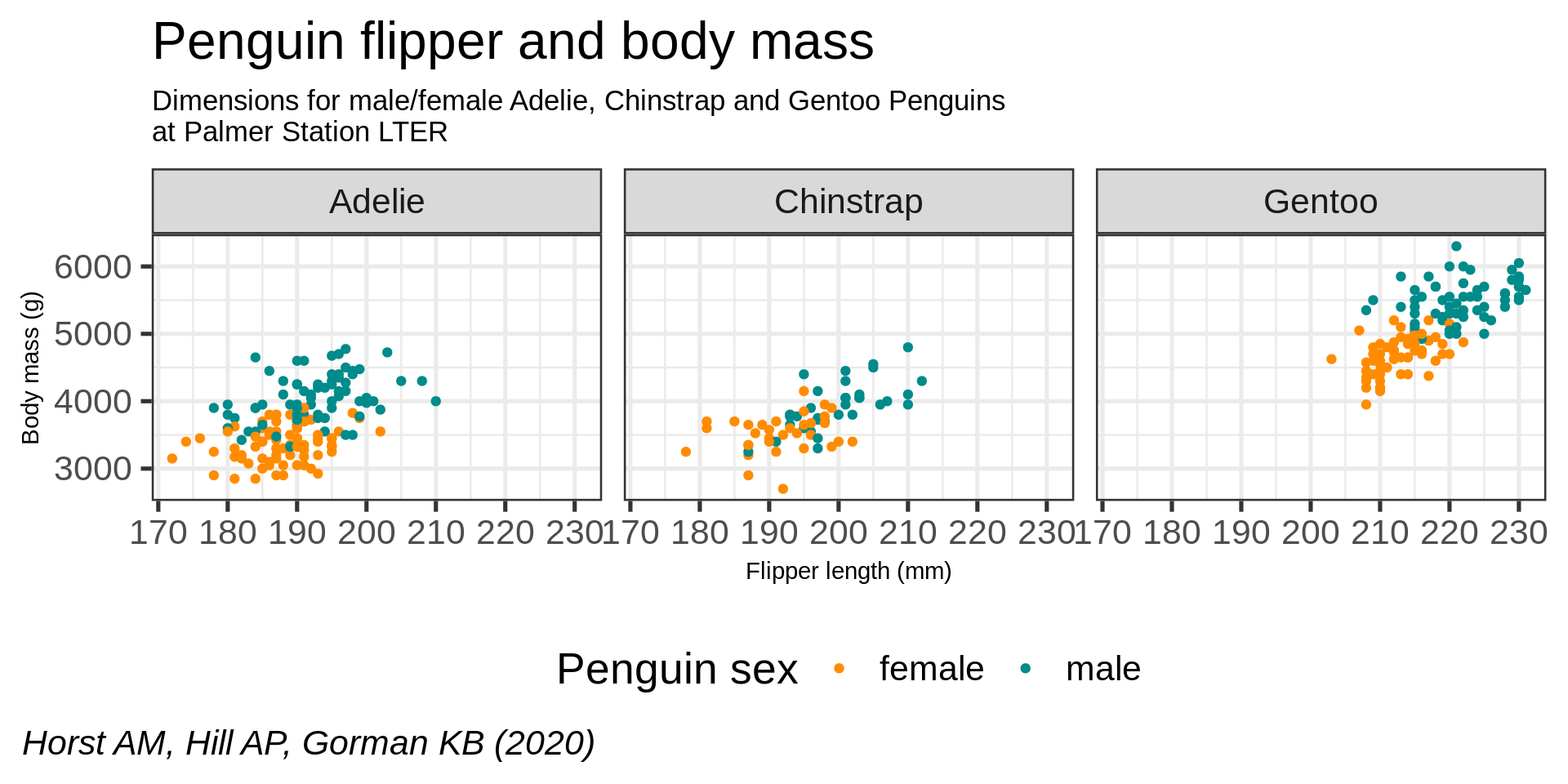
Capabilities in ggplot - tweaking the theme
gg_peng_labs +
  theme_bw() +
  theme(
    palette.colour.discrete = c("#00A4E1", "#2A8479"),
    plot.subtitle = element_text(size = 13),
    axis.title = element_text(size = 11)
  )
Capabilities in ggplot - legend
(gg_peng_labs +
  theme_bw() +
  theme(
    palette.colour.discrete = c("#00A4E1", "#2A8479"),
    plot.title = element_text(size = 24),
    plot.subtitle = element_text(size = 16),
    axis.title = element_text(size = 16),
    axis.text =  element_text(size = 14)
  ) +
  theme(legend.position = "bottom",
        legend.background = element_rect(fill = "#00A4E1"),
        legend.title =  element_text(colour = "white"),
        legend.text =   element_text(colour = "white")) -> gg_peng_themes)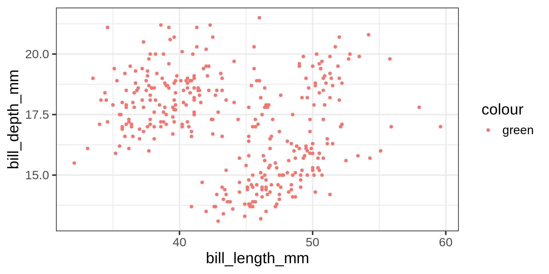
Capabilities in ggplot - facet
gg_peng_themes +
  facet_wrap(vars(species))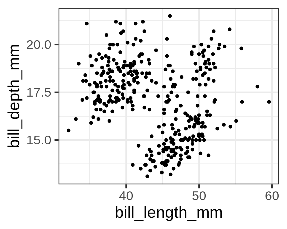
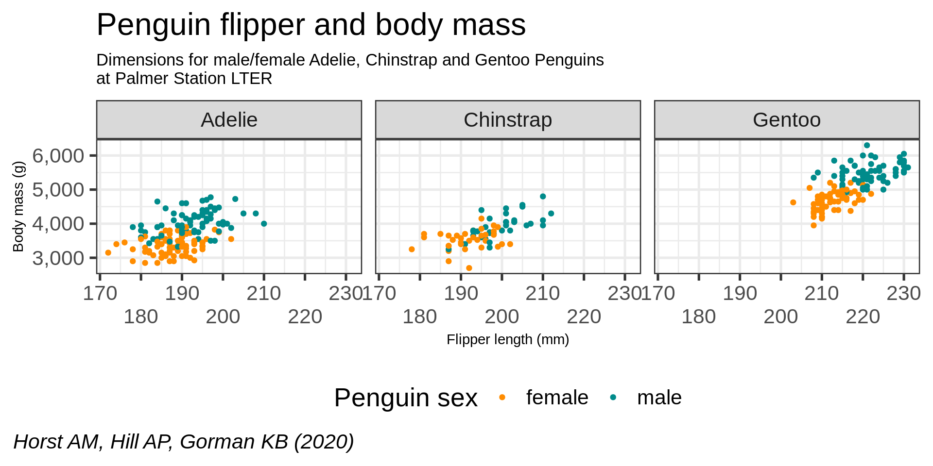
Capabilities in ggplot - scales
gg_peng_themes +
  facet_wrap(vars(species)) +
scale_y_continuous(labels = scales::label_comma()) 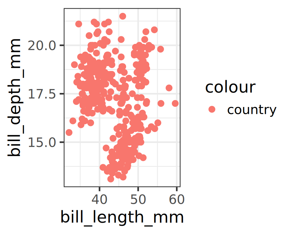
Capabilities in ggplot - coordinates
gg_peng_themes +
  facet_wrap(vars(species)) +
  scale_y_continuous(labels = scales::label_comma()) +
  coord_cartesian(xlim = c(170, 230))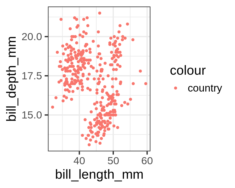
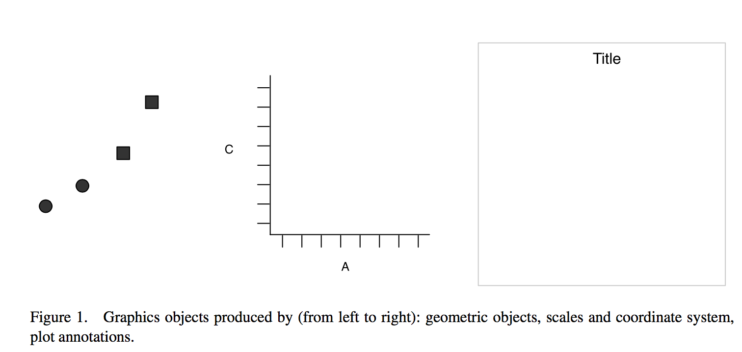
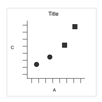
Geometric objects define the plot type to be drawn
geom_point()
geom_line()
geom_bar()
geom_violin()
geom_histogram()
geom_density()
Core parts
Other parts
They are present, it works because they have sensible default:
- Theme is
theme_grey - Coordinate is
cartesian - Facets are
disabled
Three parts are usually required
- Scales have defaults
- Geometry or Statistics at least one
- Mapping data to plot component as Aesthetics
- Data
Mapping aesthetics
Requirements
aes()map columns/variables data to aesthetics- Specific geometries (
geom) have different expectations:- univariate, one x or y for flipped axes
- bivariate, x and y like scatterplot
- Continuous or Discrete variables
- Continuous for color ➡️ gradient
- Discrete for color ➡️ qualitative
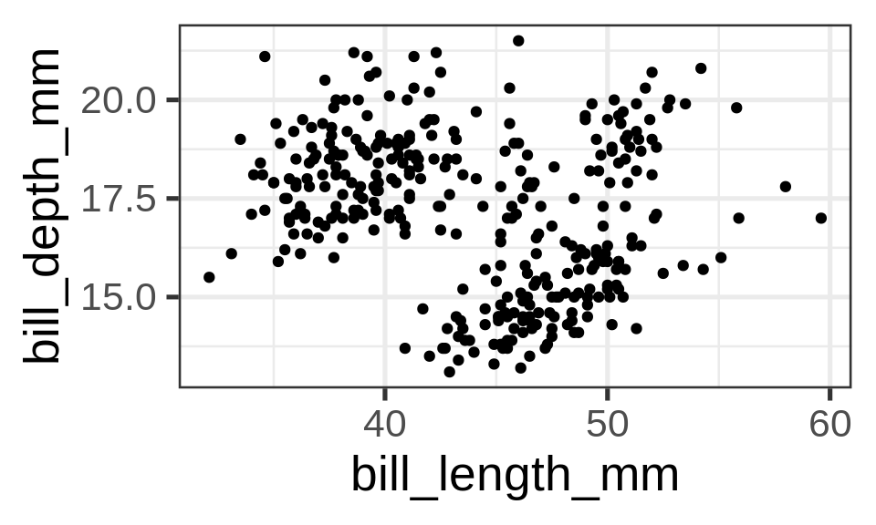
geom_point() requires both x and y coordinates
ggplot(penguins) +
  geom_point(aes(x = bill_len,
y = bill_dep))- Same as previous slide
- Without
colourmapping
Unmapped parameters
geom_point()accepts additional arguments such as thecolour- Define them to a fixed value without mapping
Important
Parameters defined outside the aesthetics aes() are applied to all data.
ggplot(penguins) +
  geom_point(aes(x = bill_len,
                 y = bill_dep),
             colour = "#00A4E1")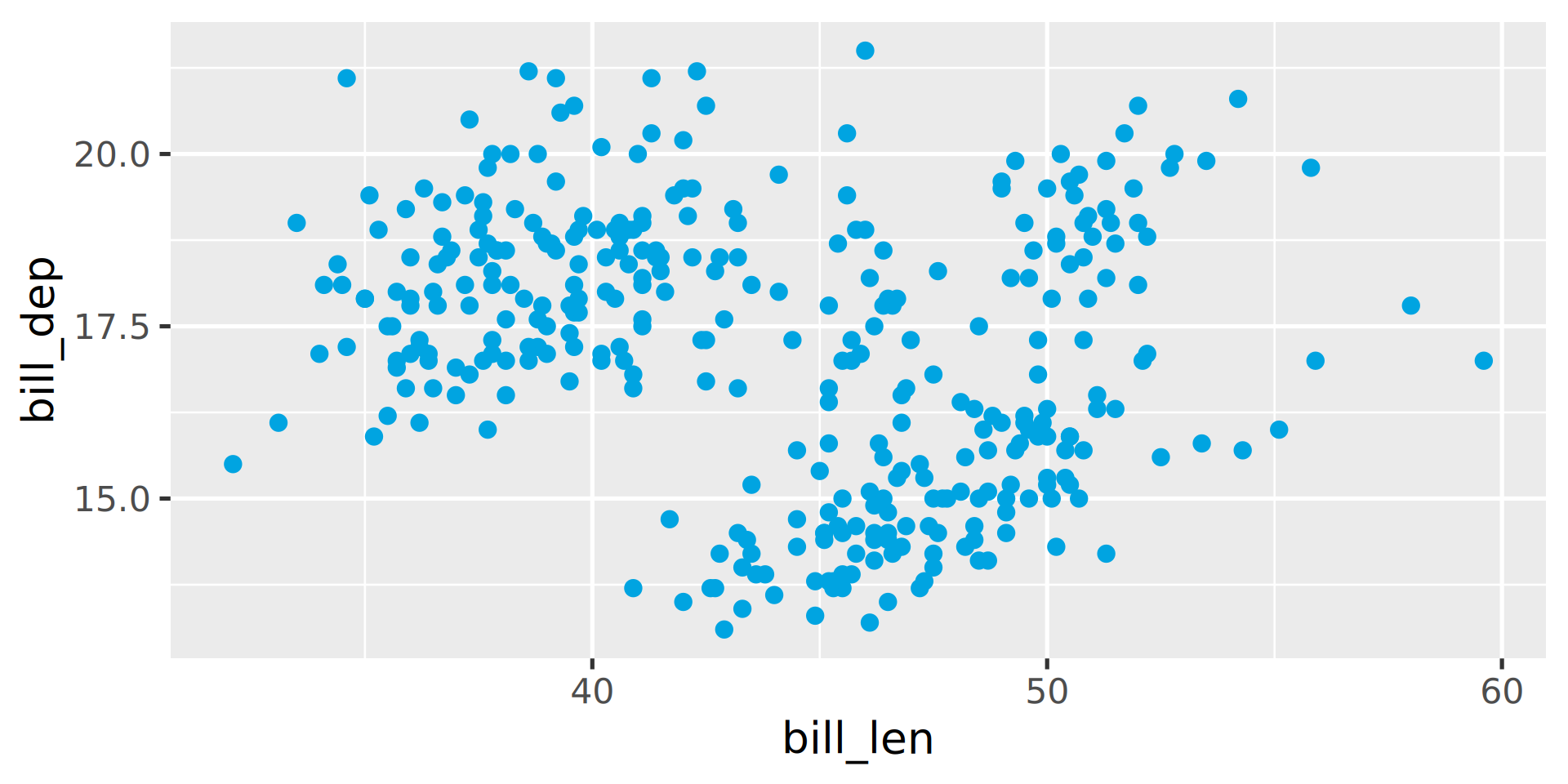
Mapped parameters
Mapped inside the aes() function
ggplot(penguins) +
  geom_point(aes(x = bill_len,
                 y = bill_dep,
                 colour = country))
Error in `geom_point()`:
! Problem while computing aesthetics.
ℹ Error occurred in the 1st layer.
Caused by error:
! object 'country' not foundPassing a column as string
ggplot(penguins) +
  geom_point(aes(x = bill_len,
                 y = bill_dep,
                 colour = "body_mass"))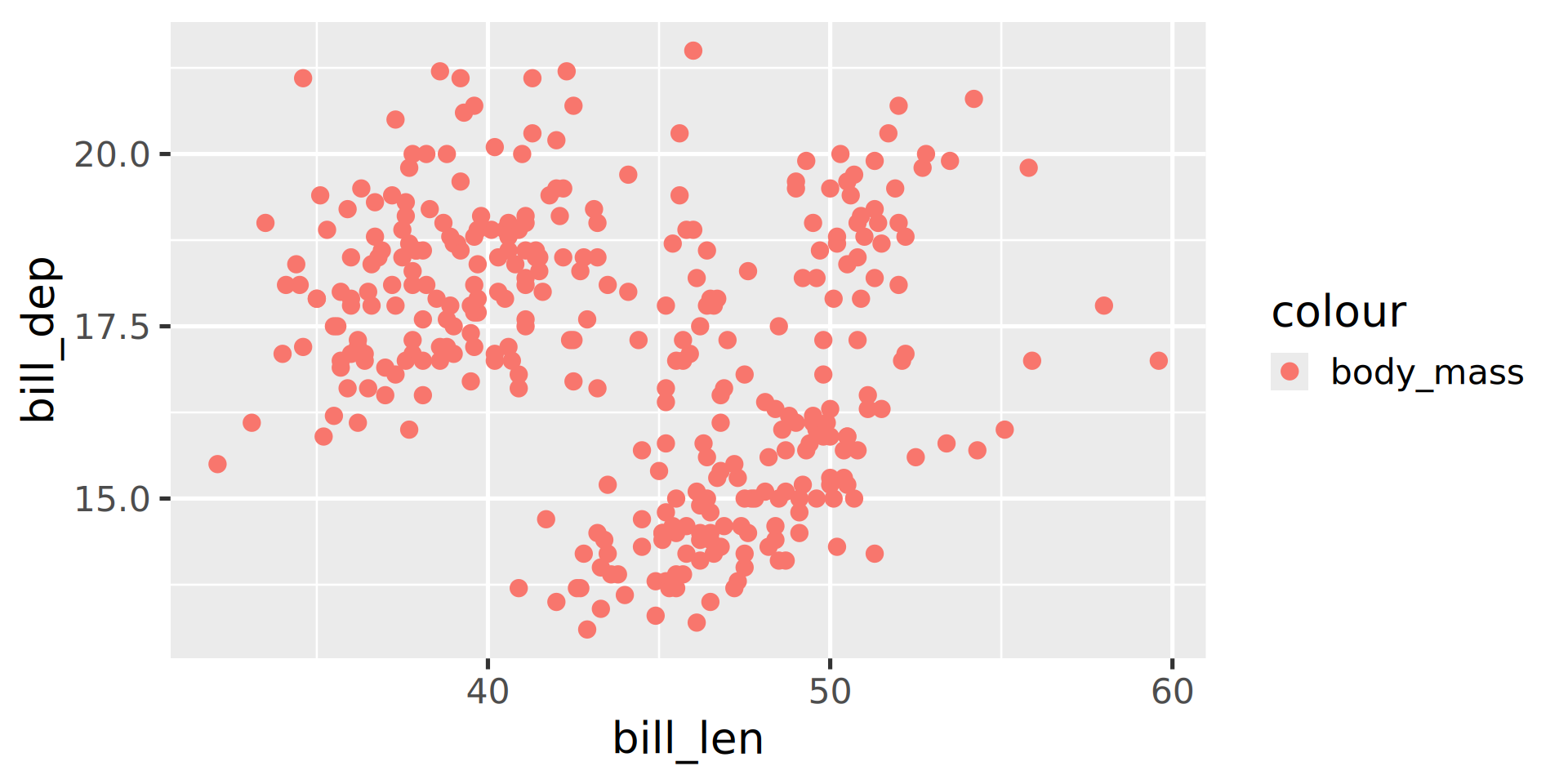
Mapping aesthetics correctly
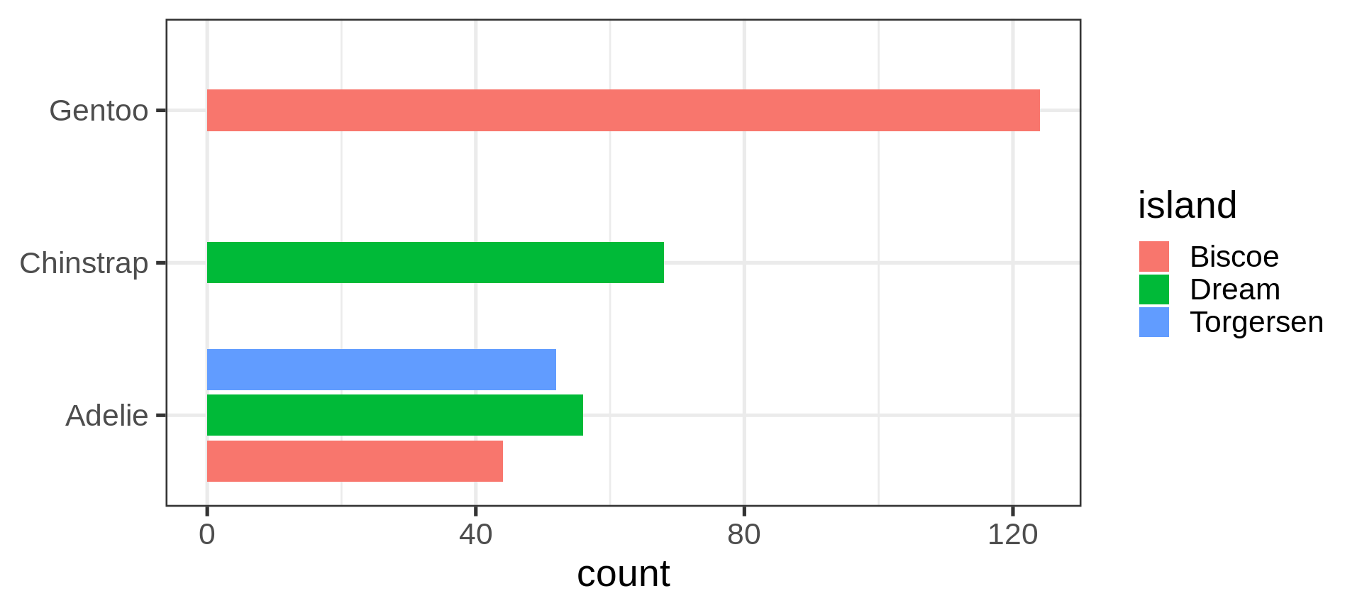
ggplot(penguins) +
  geom_bar(aes(y = species,
               fill = sex))
species and sex are 2 valid columns in penguins
Advantages:
- The legend 🟥/🟦 for free
- Missing data are highlighted in grey ⬜️
- Using
yaxis for categories eases reading
Why no string for mapping?
- Could we pass an
expression? - Which penguins are above 4 kg?
- Use
body_mass > 4000that return a boolean to find out
ggplot(penguins) +
  geom_bar(aes(y = species,
               fill = body_mass > 4000))
The expression was evaluated in penguins context.
Inheritance of arguments across parts
Compare the code and the results
Inheritance
aesthetics in ggplot() are passed on to all parts.
Specifics
aesthetics in geom_*() are specific and overwrite inherited mappings.
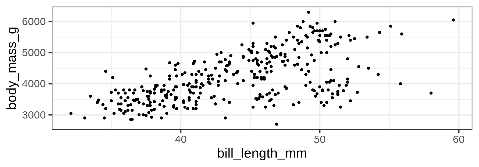
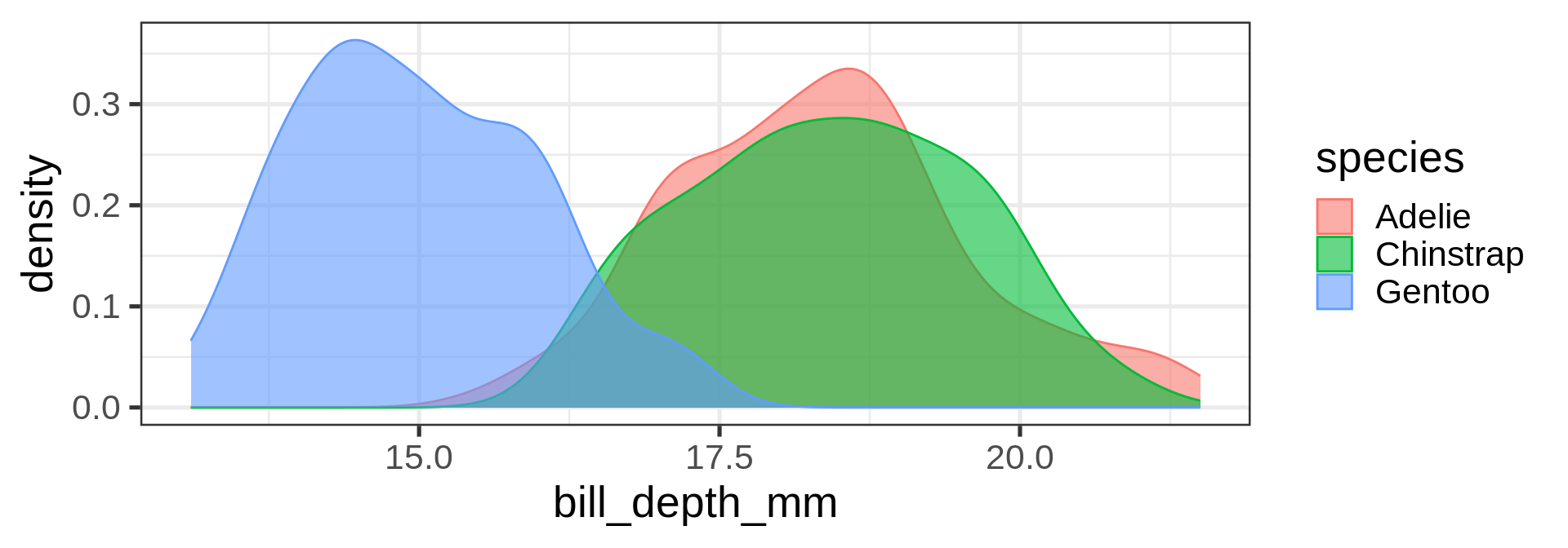
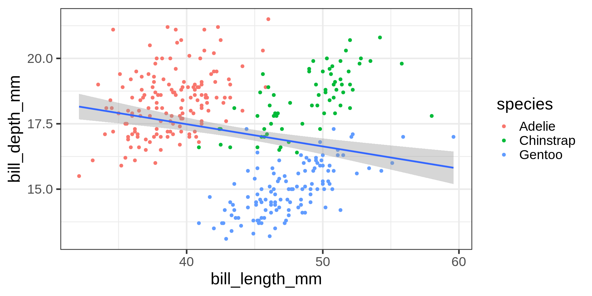
Simpson’s paradox
Statistical correlation depending on stratification.
ggplot(penguins,
       aes(x = bill_len,
           y = bill_dep)) +
  geom_point(
    aes(colour = species)) +
  geom_smooth(method = "lm", formula = 'y ~ x')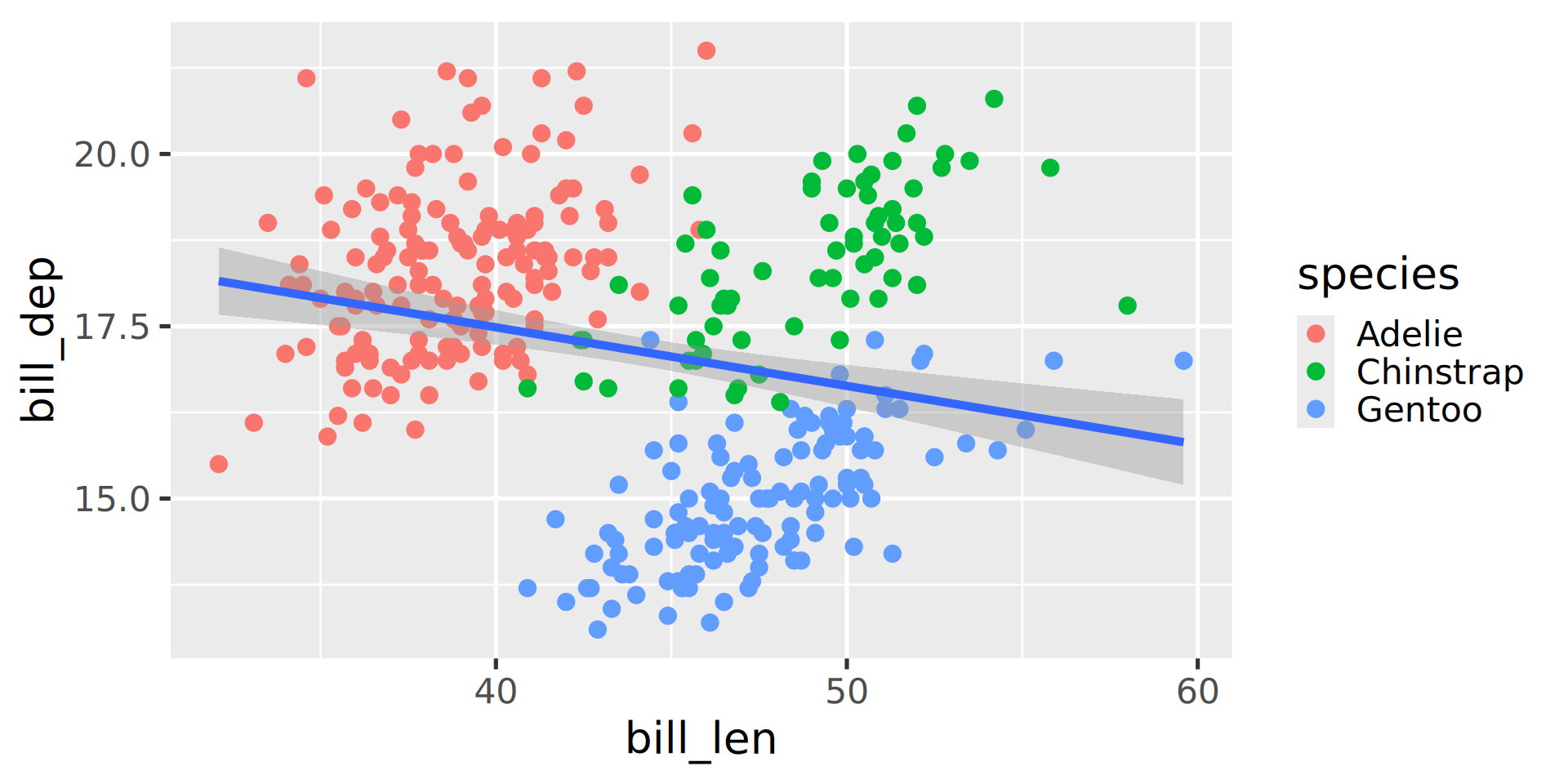
Complete data set $R^2 = $ 0.055
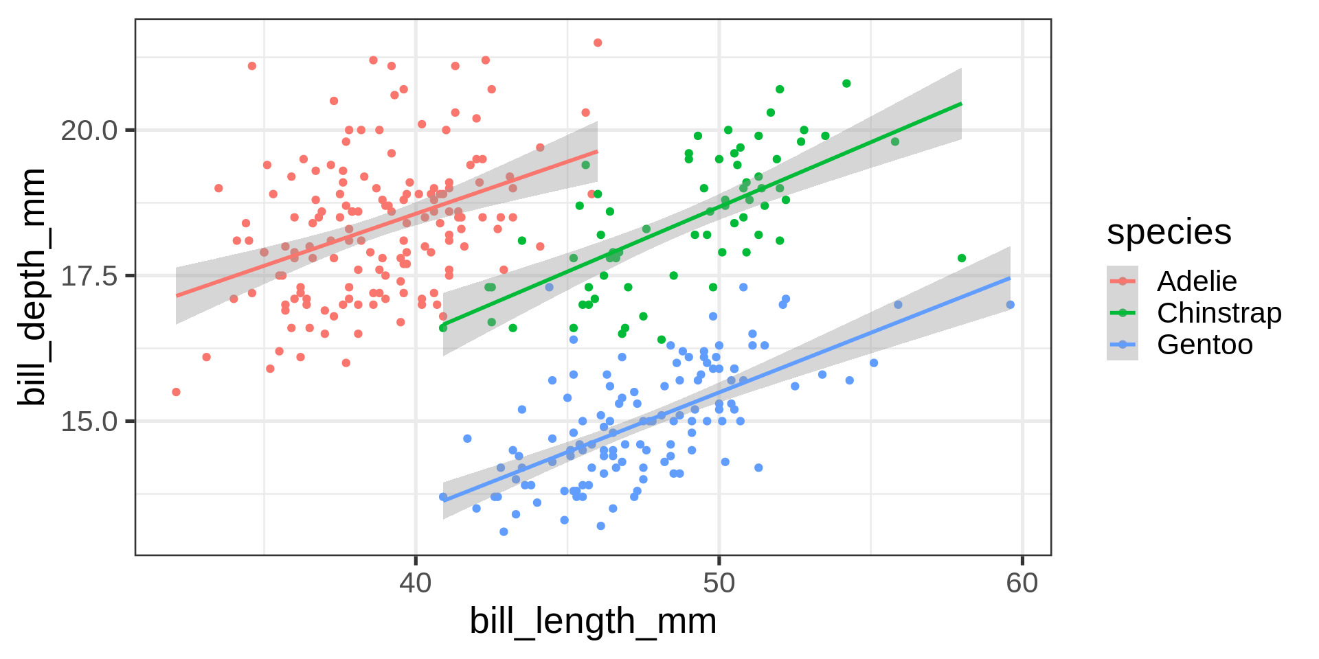
ggplot(penguins,
       aes(x = bill_len,
           y = bill_dep,
           colour = species)) +
  geom_point() +
  geom_smooth(method = "lm", formula = 'y ~ x')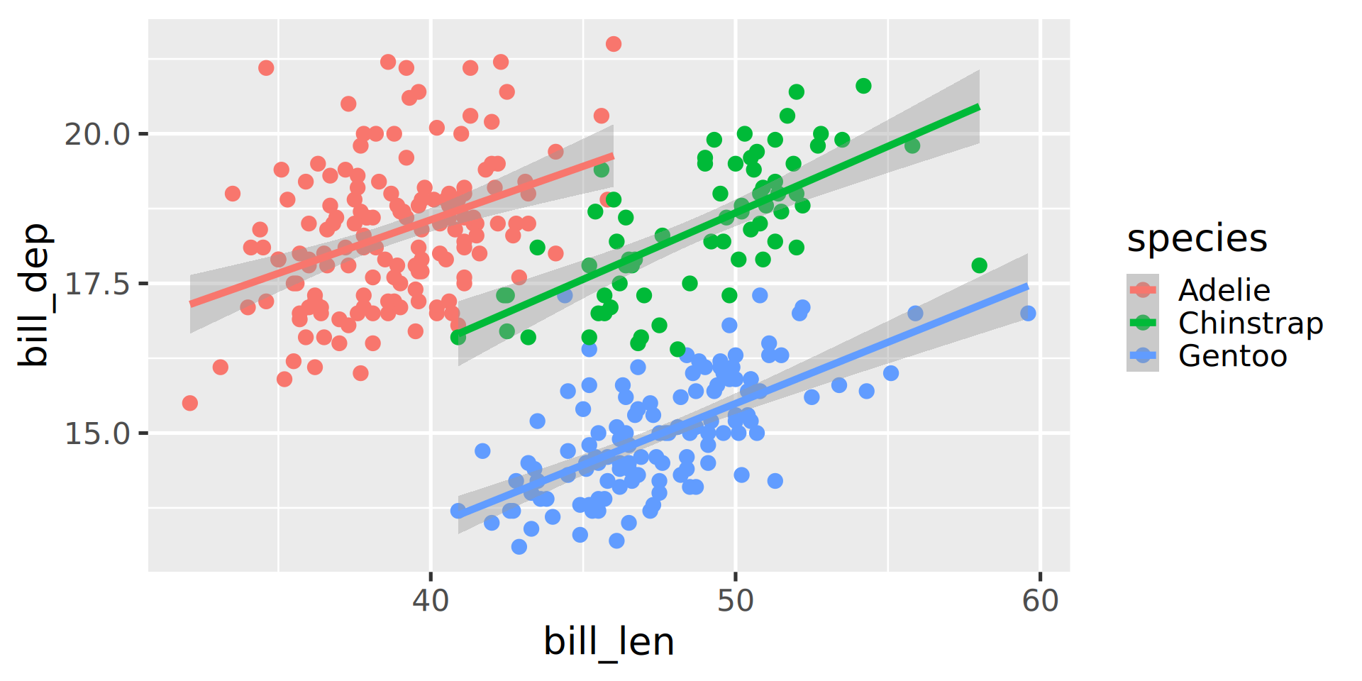
| Adelie | Gentoo | Chinstrap |
|---|---|---|
| 0.153 | 0.414 | 0.427 |
Your turn!
- Use the classroom practical.
- Install
palmerpenguinspackage if you haven’t yet - Use the
penguinsdata set and plotbill_len,bill_depandspecies. - Map the variable
islandto the aestheticsshape. - Add a regression line using a linear model.
- All dots (circles / triangles / squares) with:
- A size of
5 - A transparency of 30% (
alpha = 0.7)
- A size of
Goal
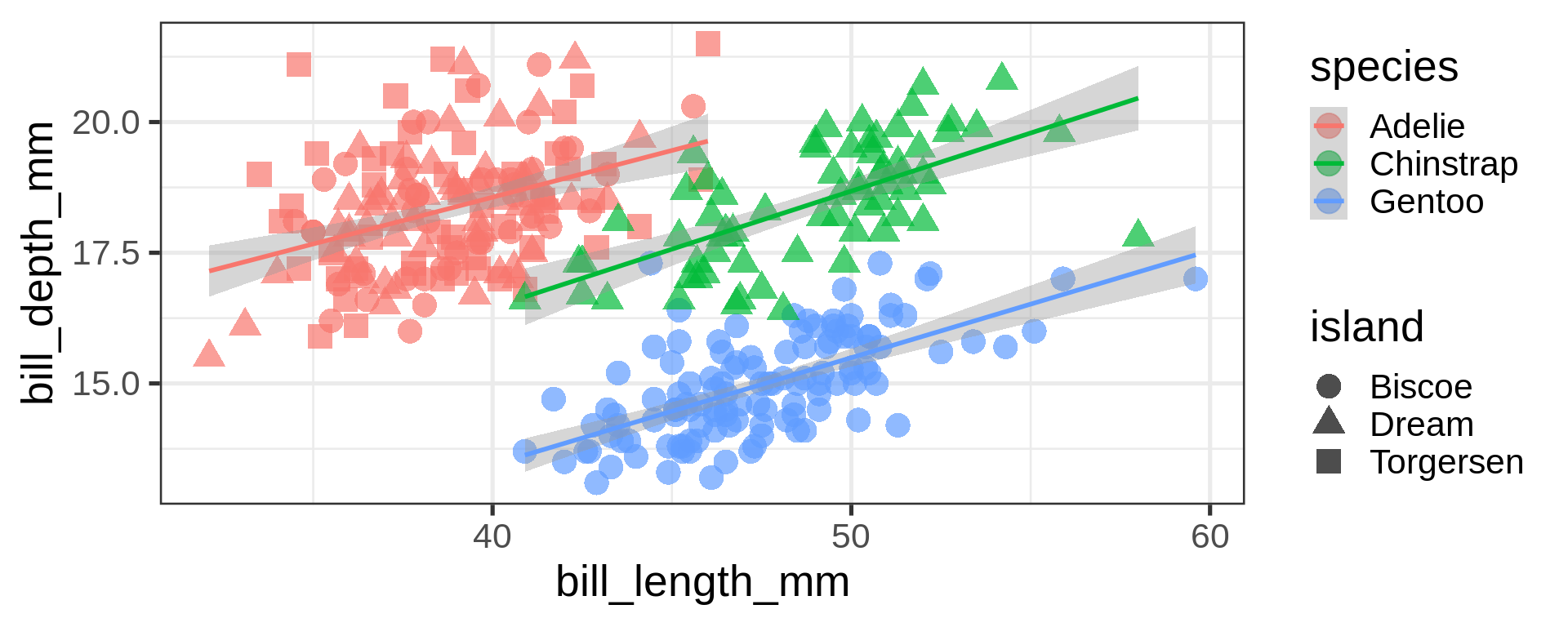
Answer:
ggplot(penguins,
       aes(x = bill_len,
           y = bill_dep,
           colour = species)) +
  geom_point(aes(shape = island),
             size = 5, alpha = 0.7) +
  geom_smooth(method = "lm",
              formula = 'y ~ x')
Statistics / geometries are interchangeable
ggplot(penguins) +
  geom_bar(aes(y = species))
Collective aesthetics
- Feels more natural since visual
- But just a preference
- Most code in the wild use
geom_bar()
ggplot(penguins) +
  stat_count(aes(y = species))
Let ggplot2 doing the stat for you
stat_count could be omitted since default
ggplot(penguins, aes(x = species)) +
  geom_bar(stat = "count")
stat_count acts on the mapped var like dplyr::count()
count(penguins, species) species n
1 Adelie 152
2 Chinstrap 68
3 Gentoo 124Count yourself geom_col()

The stat() function allows computation, like proportions
Classic counting
ggplot(penguins, aes(y = species)) +
  geom_bar(aes(x = stat(count)))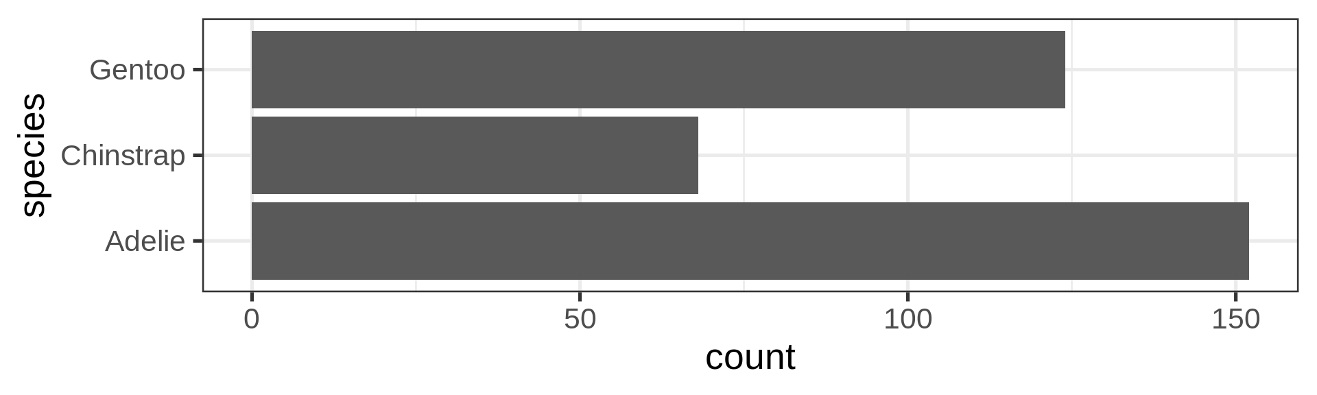
See list in help pages
ggplot(penguins, aes(y = species)) +
  geom_bar(aes(x = stat(count) / sum(count))) +
  scale_x_continuous(labels = scales::label_percent())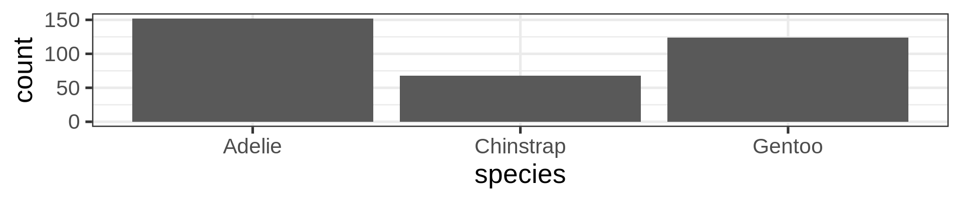
- Now compute proportions
- Bonus: get
xscale in%usingscales
Flexibility in the asthetics for flipping axes
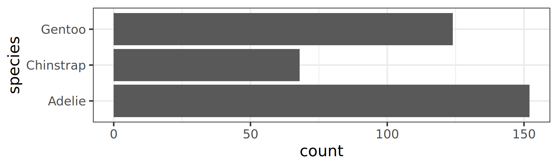
geom_bar() requires x OR y
penguins |>
  # horizontal brings readability
  ggplot(aes(y = species)) +
  geom_bar()
Cleanup plot
penguins |>
  ggplot(aes(y = species)) +
  geom_bar() +
  labs(y = NULL) +
  scale_x_continuous(expand = c(0, NA))
Annoying to see those 3 bars in disorder
Reorder the categorical variable (forcats)
Using the function fct_infreq()
library(forcats)
penguins |>
  ggplot(aes(y = fct_infreq(species) |> fct_rev())) +
  geom_bar() +
  scale_x_continuous(expand = c(0, NA)) +
  labs(title = "Palmer penguins species",
       y = NULL) +
  theme_minimal(14) +
  theme(panel.ontop = TRUE,
        # better to hide the horizontal grid lines
        panel.grid.major.y = element_blank())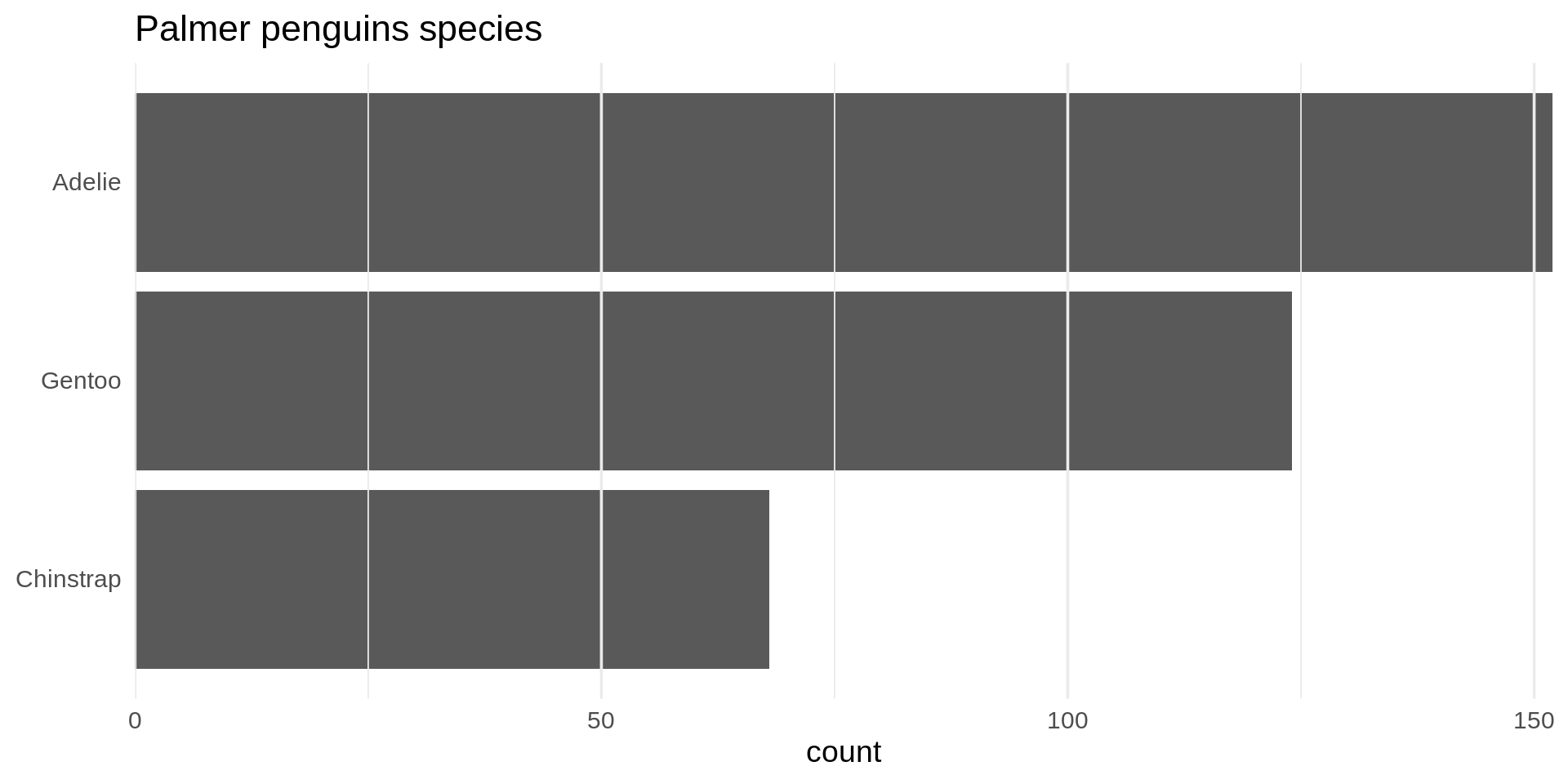
- See the new article FAQ about reordering.
Histograms
penguins |>
ggplot(aes(x = body_mass,
           fill = species)) +
  geom_histogram(bins = 35,
                 alpha = 0.7,
                 position = "identity")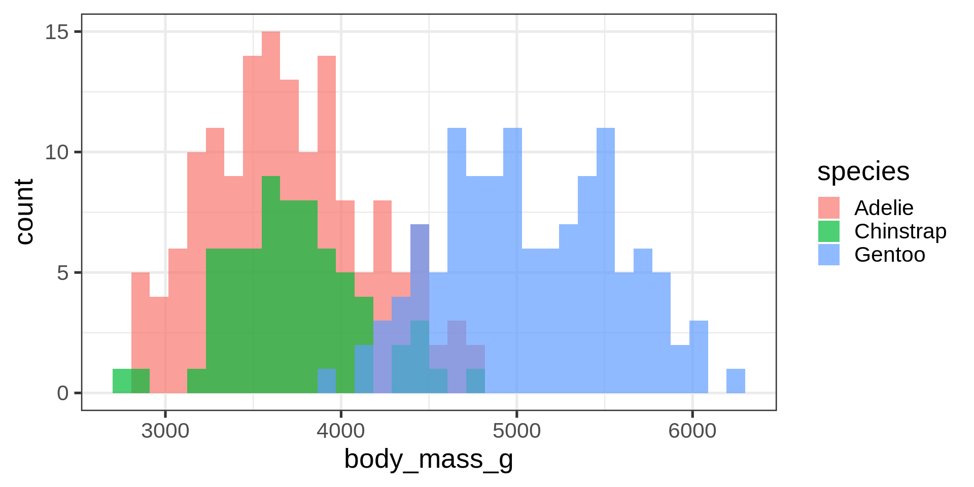
- Default
binvalue is30and will be printed out as a message - Default is
stackfor theposition. Here we overlay and use transparency
Density plots
penguins |>
ggplot(aes(x = body_mass,
           fill = species,
           colour = species)) +
  geom_density(alpha = 0.7)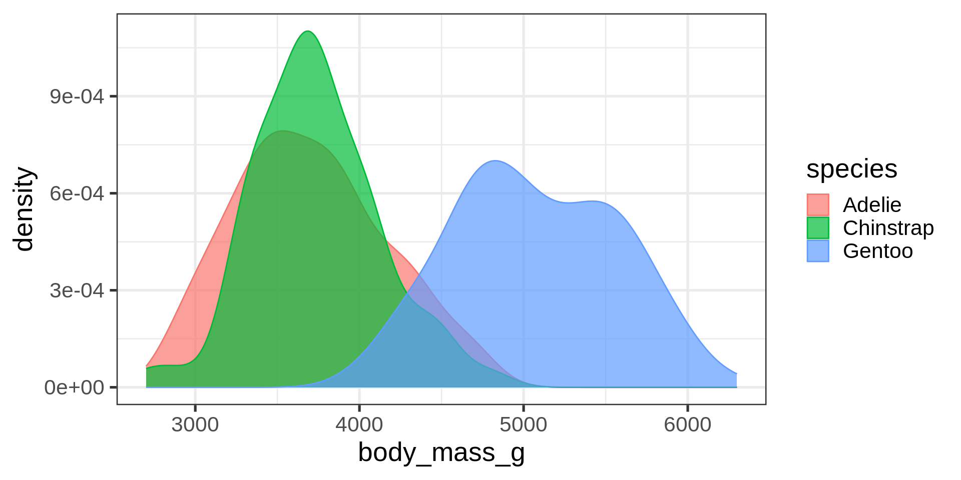
- Use both
colourandfillmapped to the same variable for cosmetic purposes
Overlay density and histogram
Naive approach: scale issue
ggplot(penguins, aes(x = body_mass)) +
  geom_histogram(bins = 30) +
  geom_density(colour = "red")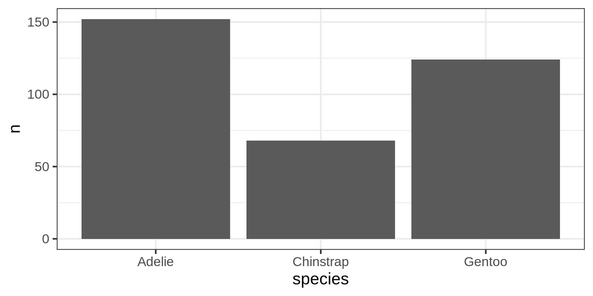
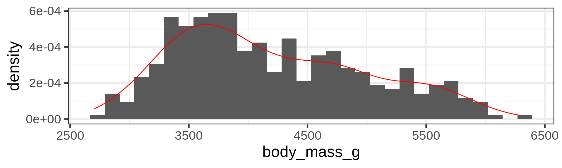
Solution: scale histogram to density one
ggplot(penguins, aes(x = body_mass)) +
  geom_histogram(bins = 30,
                 aes(y = stat(density))) + #<<
  geom_density(colour = "red")
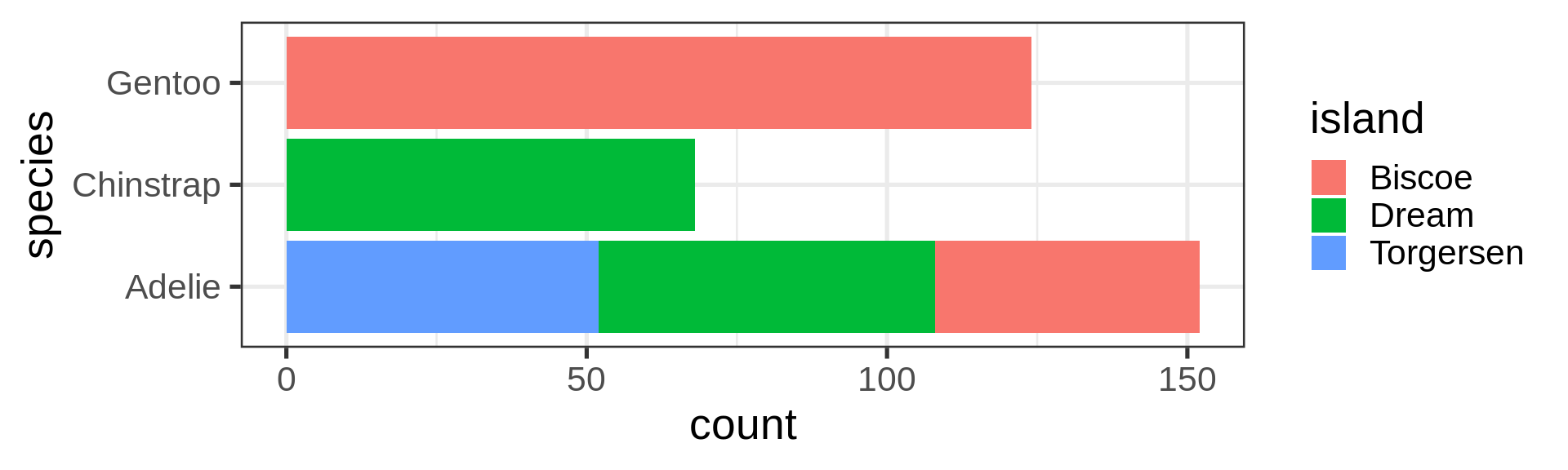
Barplot, categories
Default: position = "stack"
ggplot(penguins) +
  geom_bar(aes(y = species,
               fill = island))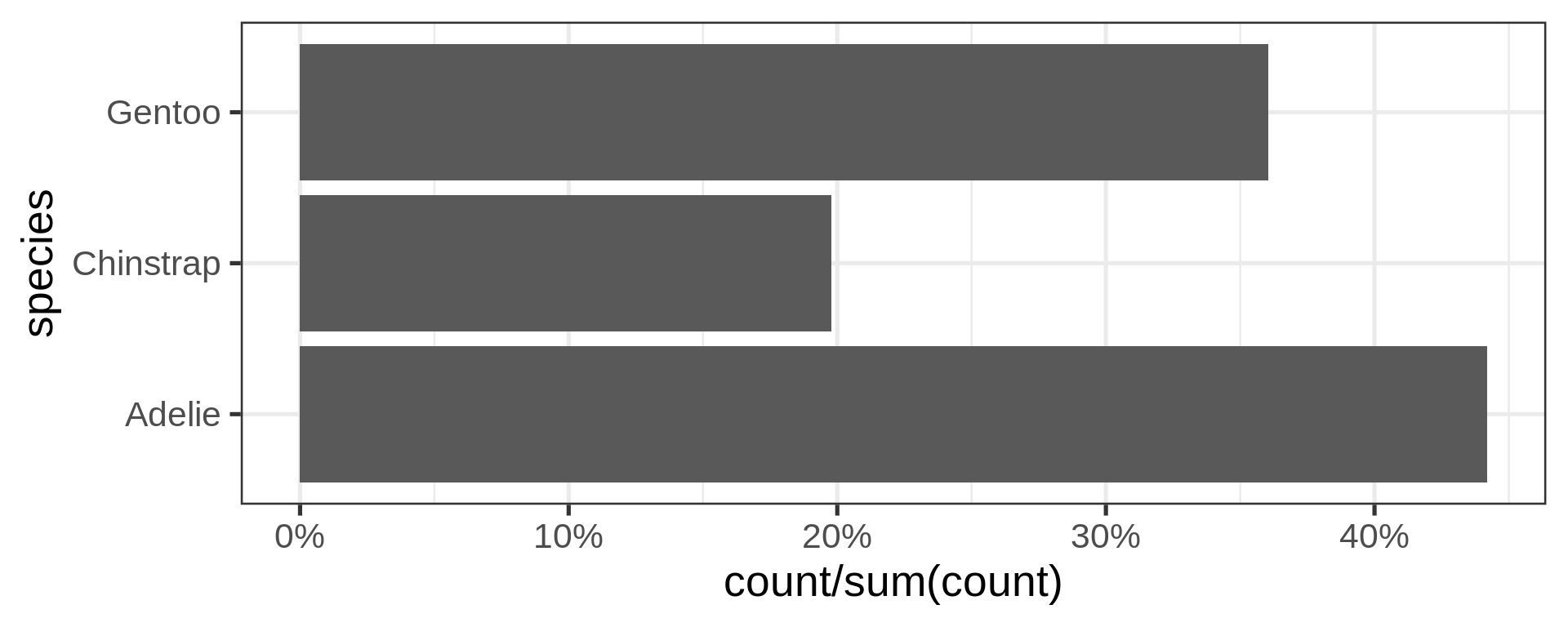
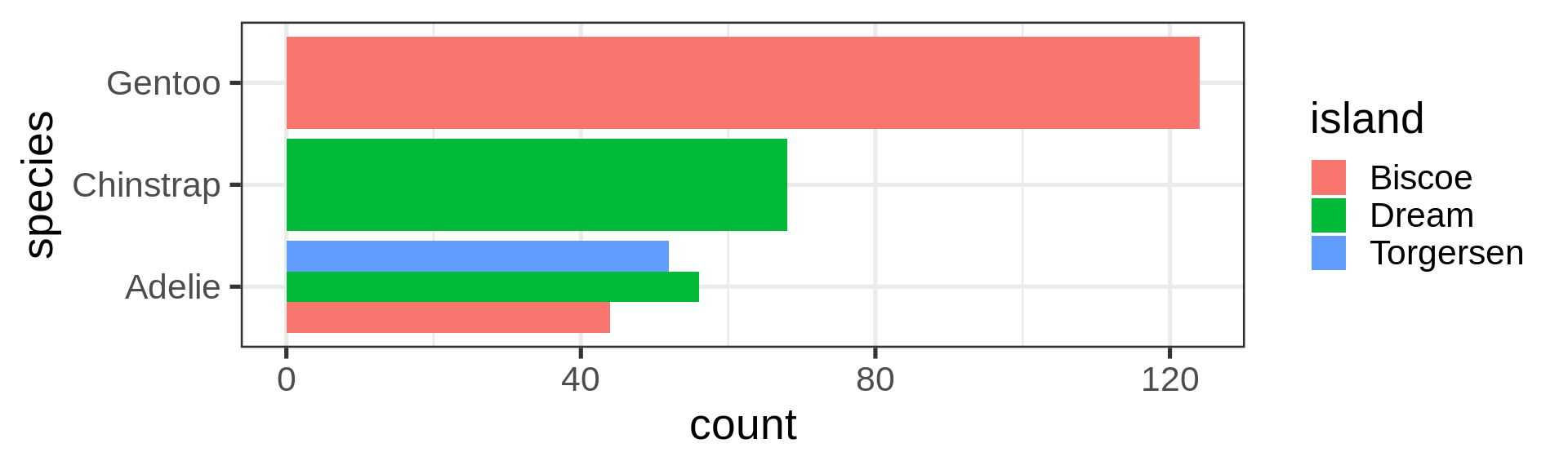
Dodging island: side by side
ggplot(penguins) +
  geom_bar(aes(y = species, fill = island),
           position = "dodge")
But global width per species is preserved
Preserve single bar
ggplot(penguins) +
  geom_bar(aes(y = species,
           fill = island),
           position = position_dodge2(preserve = "single")) +
  labs(y = NULL)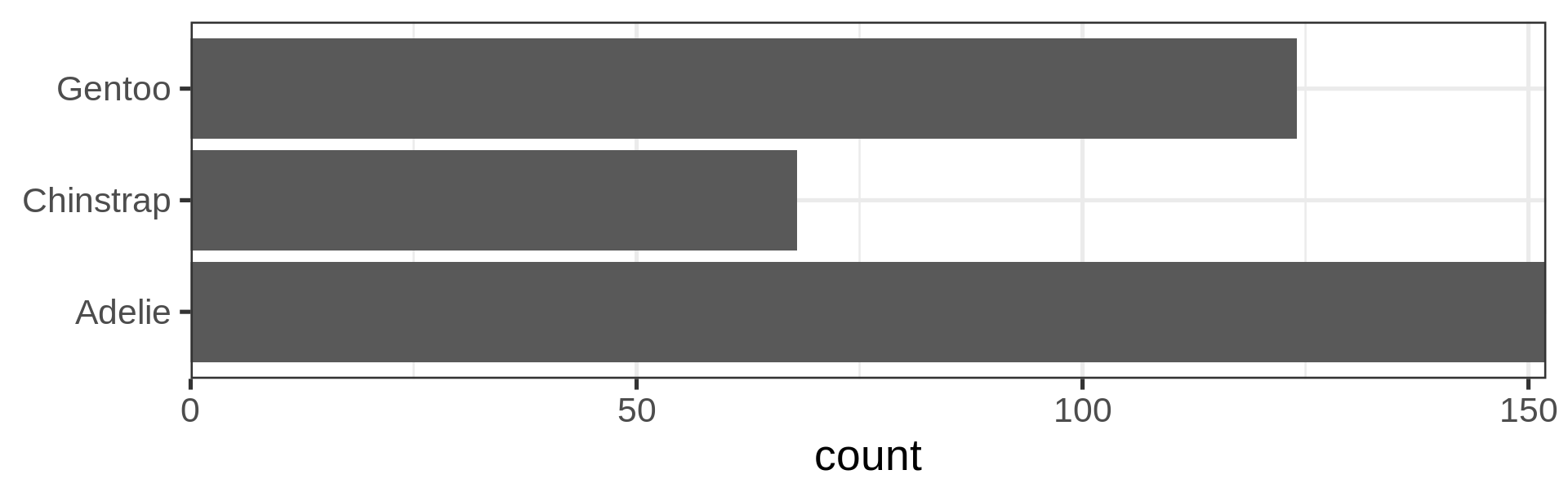
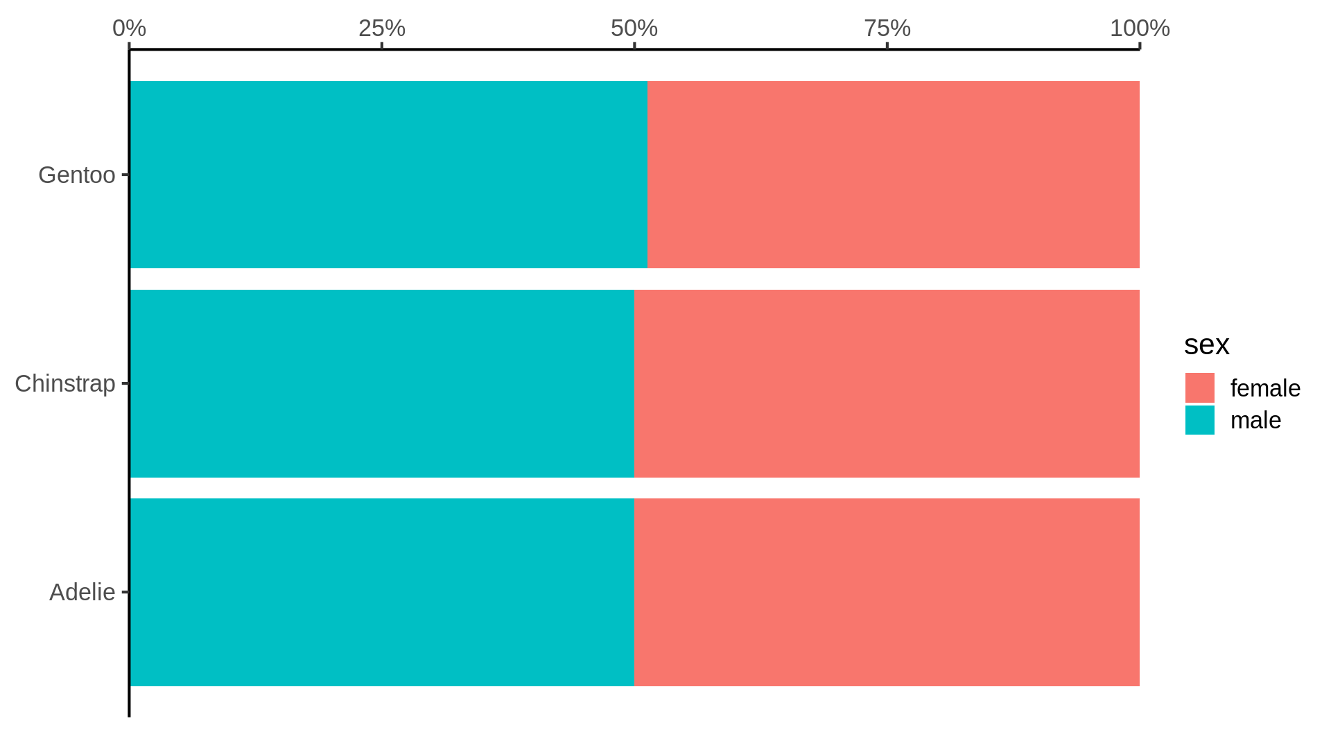
Stacked barchart for proportions
penguins |>
  drop_na(sex) |> # from tidyr
  ggplot() +
  geom_bar(aes(y = species,
               fill = sex),
           position = "fill") + #<<
  scale_x_continuous(labels = scales::label_percent(),
                     position = "top",
                     expand = c(0, 0)) +
  labs(x = NULL, y = NULL) +
  theme_classic(16)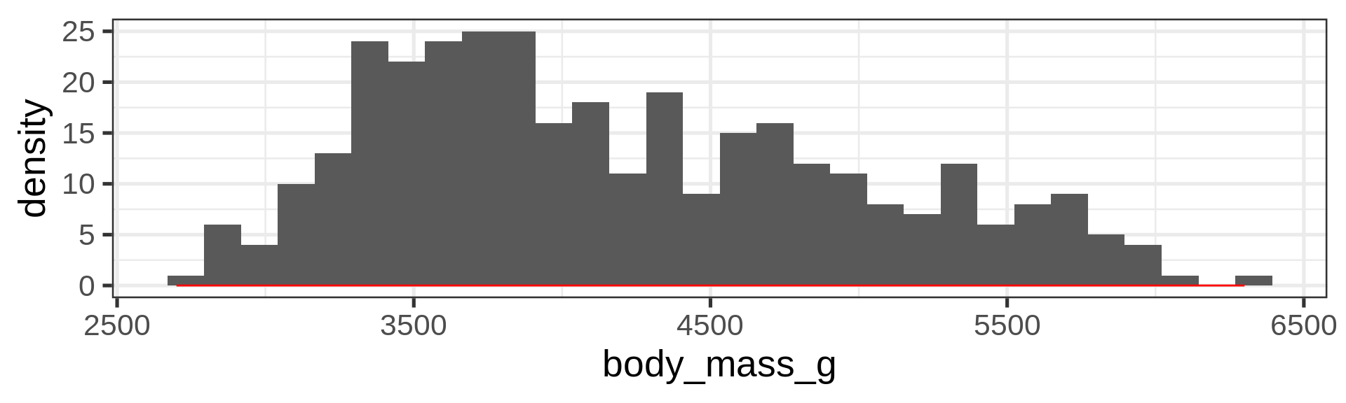
Boxplot, a continuous y by a categorical x
ggplot(penguins) +
  geom_boxplot(aes(y = body_mass,
                   x = species))
Note
geom_boxplot() is assessing that:
body_massis continuousspeciesis categorical/discrete
Boxplot, dodging by default
penguins |> # alternative to tidyr::drop_na()
  tidyr::drop_na() |>
  ggplot() +
  geom_boxplot(aes(y = body_mass,
                   x = species,
                   fill = sex))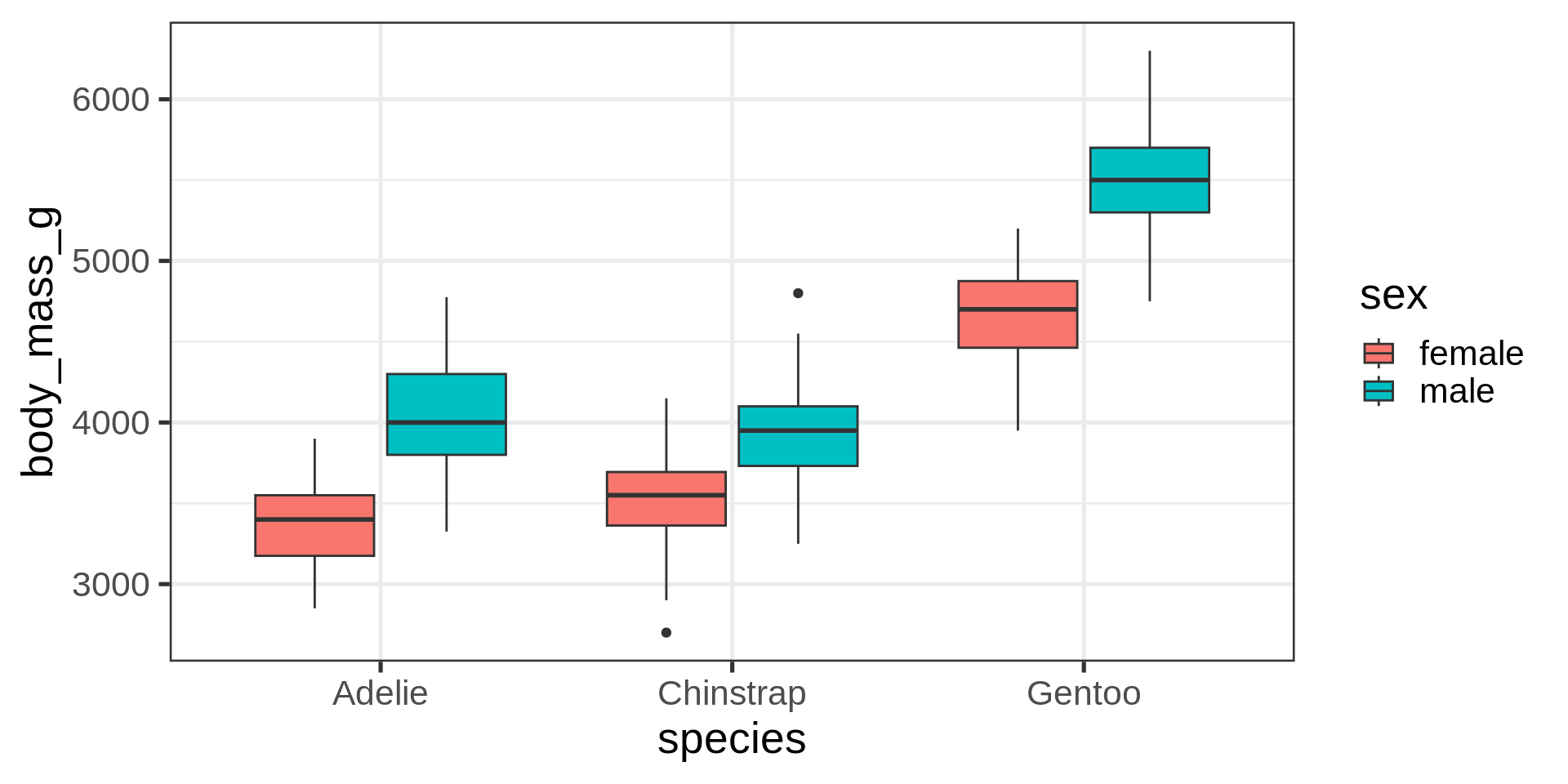
Filter out NA to avoid additional category for missing data.
Better: violin and jitter
Show the data
penguins |>
  filter(!is.na(sex)) |>
  # define aes here for both geometries
  ggplot(aes(y = body_mass,
             x = species,
             fill = sex,
             # for violin contours and dots
             colour = sex
  )) +        # very transparent filling
  geom_violin(alpha = 0.1, trim = FALSE) +
 geom_point(position = position_jitterdodge(dodge.width = 0.9),
#  geom_point(position = position_dodge2(width = 0.9 , preserve = "total", padding = 0.005),

             alpha = 0.5,
             # don't need dots in legend
             show.legend = FALSE)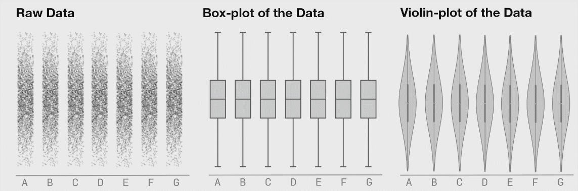
Coding mistake
What is wrong with this code?
Think about inherited aesthetics!
penguins |>
  ggplot() +
  geom_point(aes(x = bill_len,
                 y = body_mass)) +
  geom_smooth(method = "lm")
Error in `geom_smooth()`:
! Problem while computing stat.
ℹ Error occurred in the 2nd layer.
Caused by error in `compute_layer()`:
! `stat_smooth()` requires the following missing
aesthetics: x and y.Inheritance of aesthetics in main ggplot()
penguins |>
  ggplot(aes(x = bill_len,
             y = body_mass)) +
  geom_point() +
  geom_smooth(method = "lm", se = FALSE)