Geographical data

Maps

Cédric Laczny

MADS6

Wednesday, 1 April 2026

Introduction

Maps

Learning objectives

Paths to simple maps with ggplot2
Limitations of default maps
Projected maps with standard geographic packages
- spatial features with sf
Learn about the Coordinate Reference System (CRS)
Drawing choropleths

Material

maps and ggplot2 for simple maps
sf for spatial maps
rnaturalearth for sf compatible data sources
Claus O. Wilke’s Data visualisation guides
Geocomputating with R

Basic maps

But first: why do maps matter?

Where do people live?
How does income vary geographically?
Where are risks (flooding, pollution)?
etc.

They provide a readily accessible way of visualizing spatial data and questions can be answered with spatial data. IF done right!

Basic map data in R

Basics from `maps`

library(maps) # R Built-in library
iso3166|> # ISO 3166 country codes (2 or 3 letters) and sovereignty.
  slice_sample(n = 10) |>
  gt()

a2	a3	ISOname	mapname	sovereignty
GQ	GNQ	Equatorial Guinea	Equatorial Guinea	Equatorial Guinea
EH	ESH	Western Sahara	Western Sahara	Western Sahara
BA	BIH	Bosnia and Herzegovina	Bosnia and Herzegovina	Bosnia and Herzegovina
SB	SLB	Solomon Islands	Solomon Islands	Solomon Islands
ES	ESP	Spain	Spain	Spain
DK	DNK	Denmark	Denmark	Denmark
MR	MRT	Mauritania	Mauritania	Mauritania
PY	PRY	Paraguay	Paraguay	Paraguay
CK	COK	Cook Islands	Cook Islands	Cook Islands
SJ	SJM	Svalbard and Jan Mayen	Norway:Svalbard	Norway

Basic maps with `ggplot`

Using `maps`

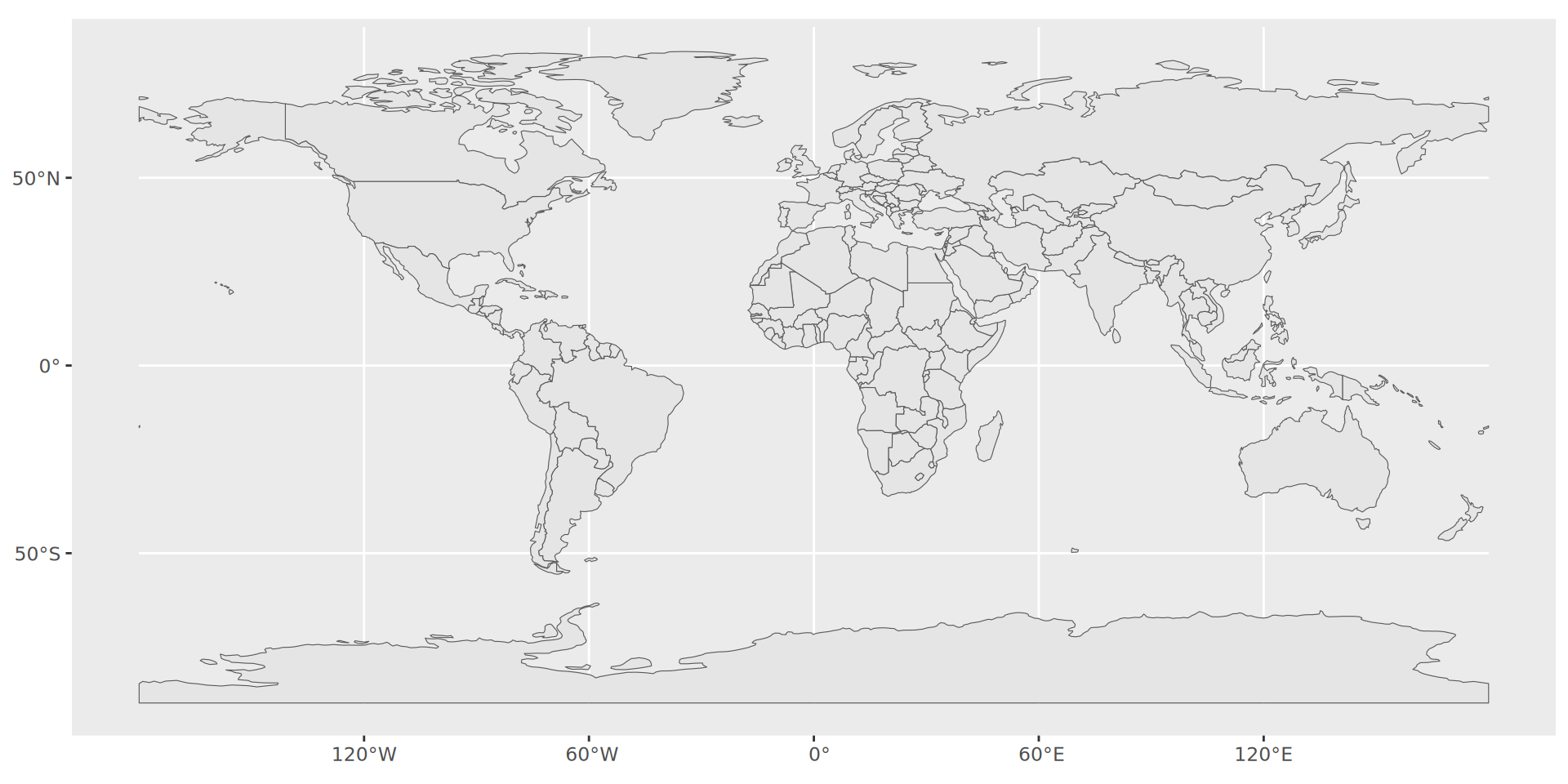
ggplot(world) + # from maps package
  geom_sf() # To draw spatial data structures and projections; handles projection but more on that later.

Basic maps with `ggplot`

`ggplot` knows the world

library(ggplot2)

gworld <- ggplot2::map_data("world") # ggplot "version" of the world
luxembourg <- map_data("world", region = "Luxembourg")

gworld |> 
  filter(region == "Luxembourg") |> 
  slice_sample(n = 10)

       long      lat group order     region subregion
1  6.110058 50.12378   958 59749 Luxembourg      <NA>
2  5.787988 49.75889   958 59737 Luxembourg      <NA>
3  5.823438 49.50508   958 59730 Luxembourg      <NA>
4  6.484766 49.70781   958 59715 Luxembourg      <NA>
5  6.493750 49.75439   958 59714 Luxembourg      <NA>
6  6.054786 50.15430   958 59747 Luxembourg      <NA>
7  5.740820 49.85718   958 59740 Luxembourg      <NA>
8  5.735253 49.87564   958 59741 Luxembourg      <NA>
9  6.242187 49.49434   958 59722 Luxembourg      <NA>
10 5.815430 49.55381   958 59732 Luxembourg      <NA>

… which we can easily visualise

ggplot(gworld) +
  geom_line(aes(x = long, y = lat))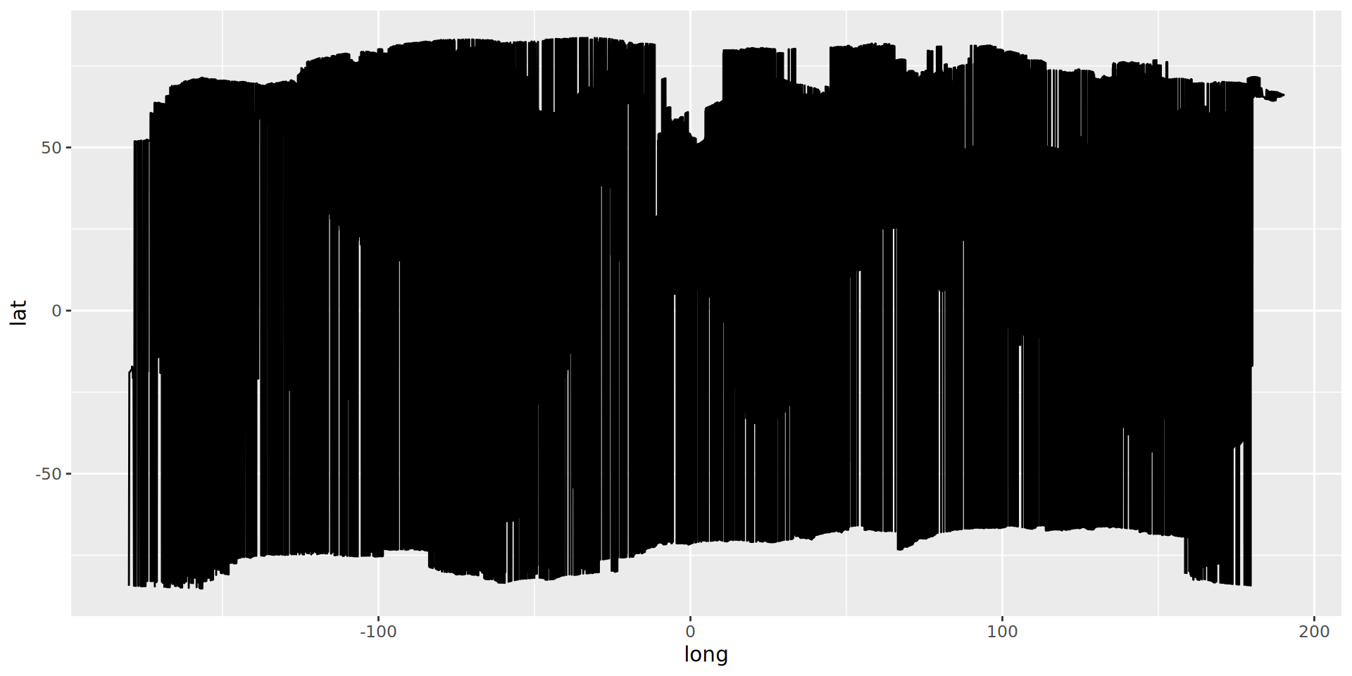

Basic maps with `ggplot`

`ggplot` knows the world

library(ggplot2)

gworld <- map_data("world")

gworld |> 
  slice_sample(n = 10)

          long        lat group order    region  subregion
1   102.461716  13.015039   910 57660  Cambodia       <NA>
2   -73.975975  18.601416   689 46481     Haiti       <NA>
3   100.324318   7.644189  1413 88259  Thailand       <NA>
4     9.916016  27.785692   486 35694   Algeria       <NA>
5  -160.992386  58.561039  1556 95672       USA     Alaska
6    18.901075  45.907616  1383 86116    Serbia       <NA>
7    26.620214  55.679638   216 11628   Belarus       <NA>
8   134.100006  -3.799707   780 48741 Indonesia Irian Jaya
9   -74.368462 -45.735840   407 27340     Chile         21
10  144.005463  44.116650   896 55666     Japan   Hokkaido

… which we can easily visualise if groups are respected

ggplot(gworld) +
  geom_polygon(aes(x = long, y = lat, group = group))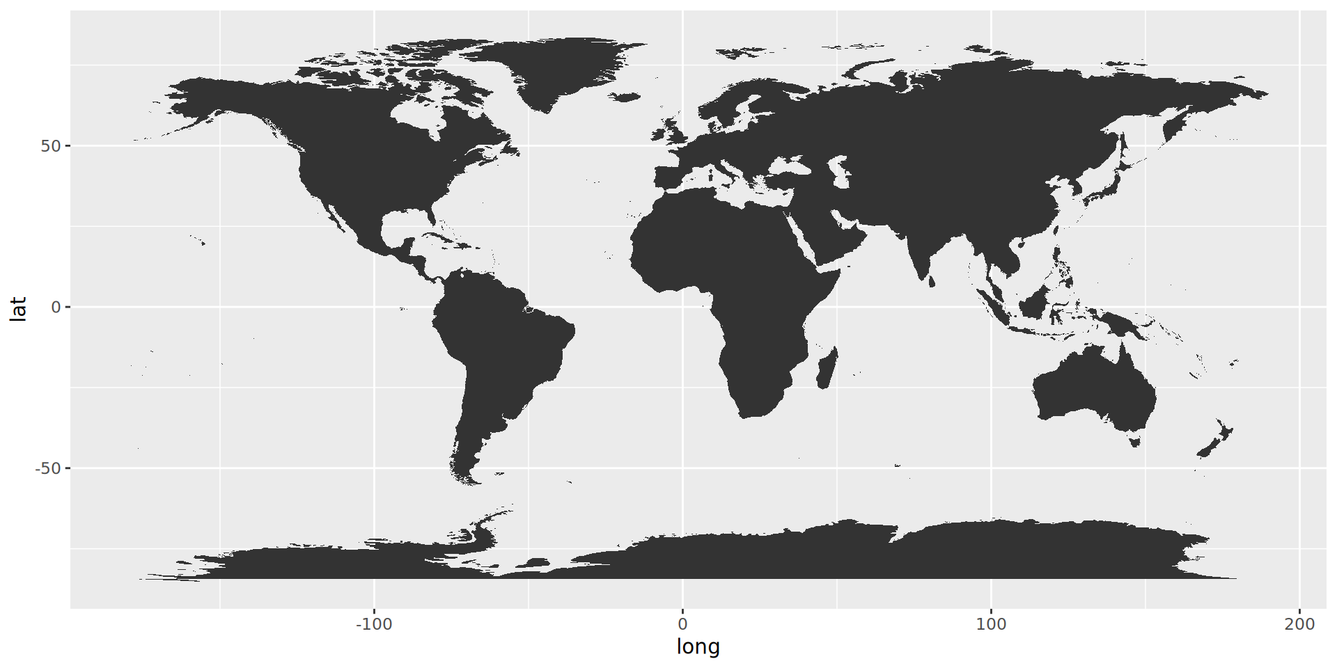

`geom_polygon()` give us countries

ggplot(gworld) +
  geom_polygon(aes(x=long, 
                   y = lat, 
                   group = group),
               color = "white")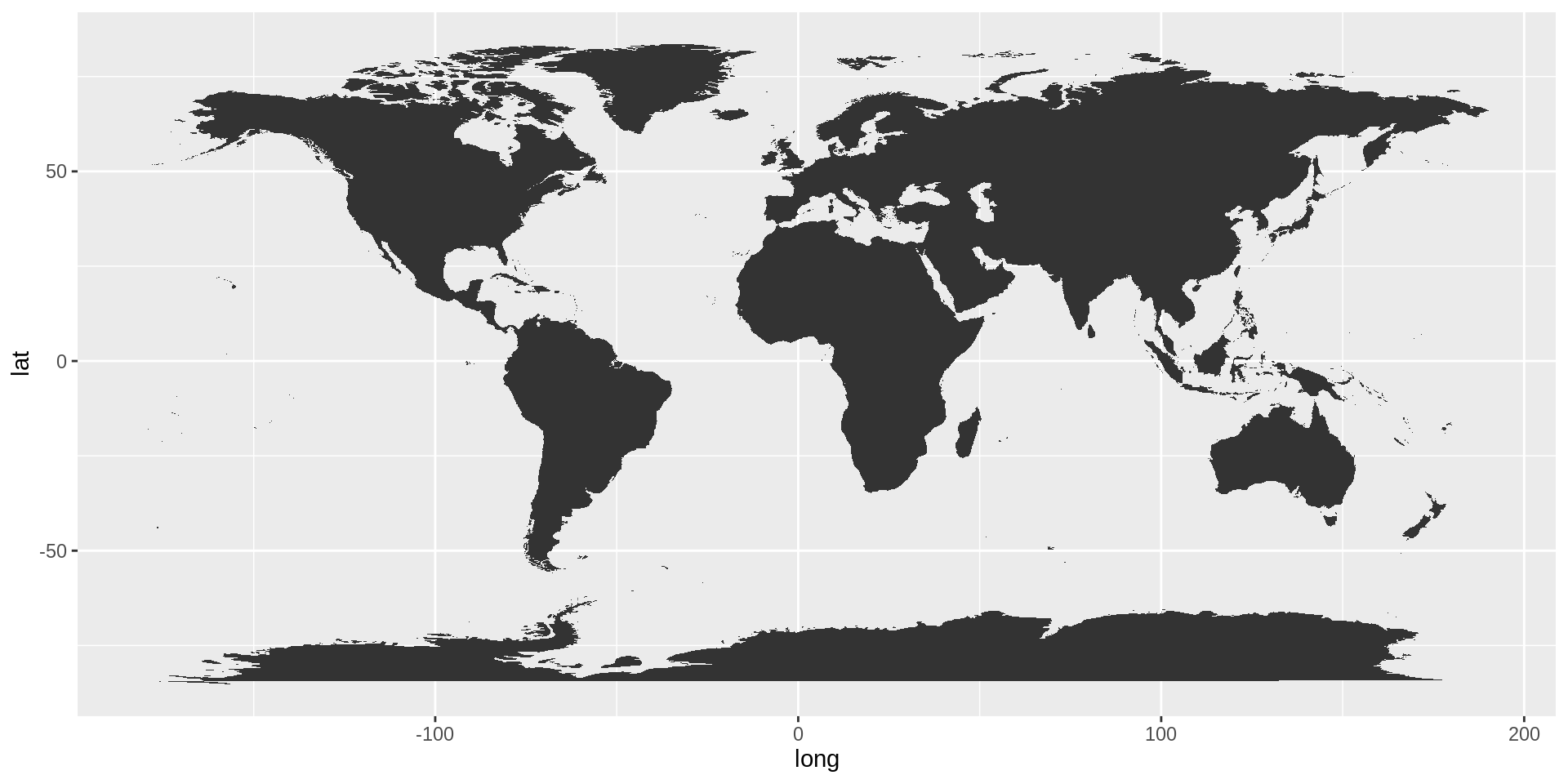

`geom_map()`

ggplot(gworld) +
  geom_map(map = gworld, 
           data = gworld,
           aes(map_id = region,
               fill = region)) +
  expand_limits(x = gworld$long, y = gworld$lat) +
  guides(fill = "none") +
  scale_fill_discrete_qualitative(palette = "Dark 2")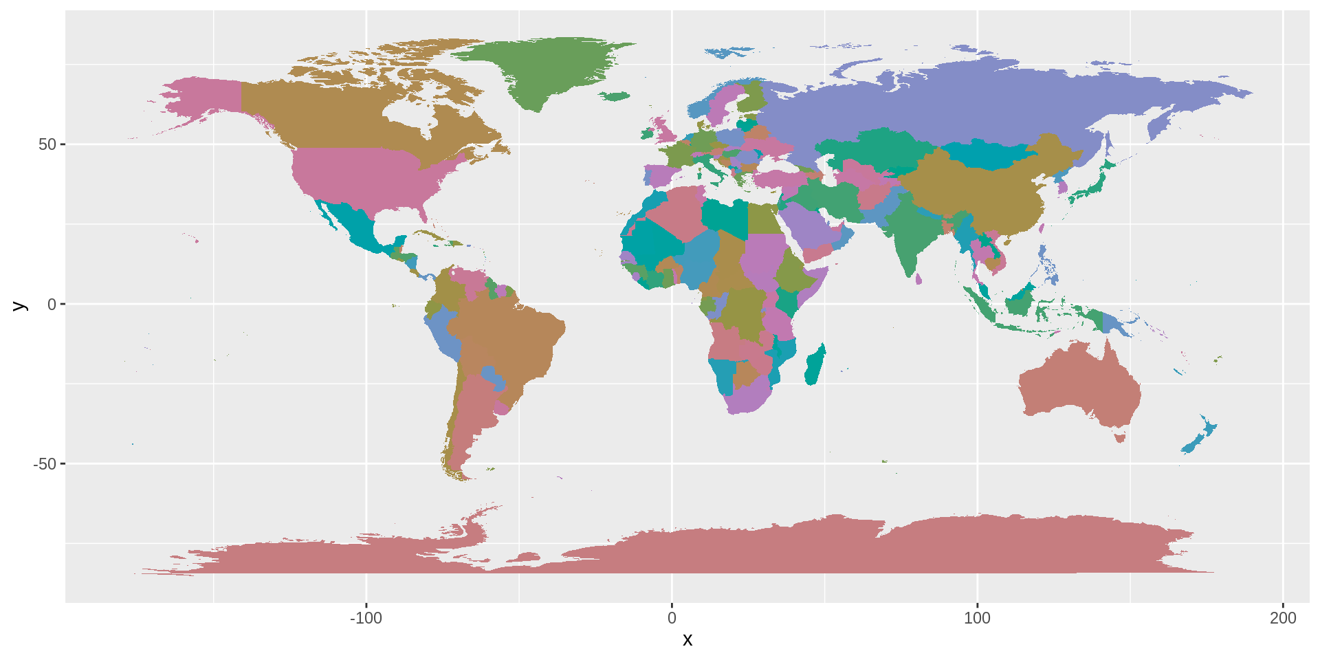

Caution

map() != mapping()

Great map, but input data is limited. And geom_map() is barely explained.

Zooming in on Luxembourg

mno_1020 = data.frame(long = c(5.9479), 
                      lat = c(49.5037))

ggplot() +
  geom_map(data = gworld,
    map = gworld,
           aes(map_id = region,
               fill = region),
           color = "black") +
  geom_point(data = mno_1020, 
    aes(long, lat),
    color = "white",
    size = 3.5) +
    # add repelled labels with lines
  geom_label_repel(data = mno_1020,
                  aes(x = long, y = lat, label = "MNO"),
                  fill="black",
                  color = "white",
                  size = 3,
                  label.r = unit(0.25, "lines"), # rounded corners
                  label.size = 0.4, # border thickness
                  segment.color = "white",
                  segment.size = 0.7,
                  nudge_y = 0.3, # Keep label above
                  force=5, # Keep label further away
                  box.padding = 1,
                  point.padding = 1) +
  expand_limits(x = gworld$long, y = gworld$lat) +
  coord_cartesian(xlim = c(5.5, 6.75), 
                  ylim = c(48.5, 51)) + 
  scale_fill_discrete_qualitative(palette = "Dark 2") +
  guides(fill = "none")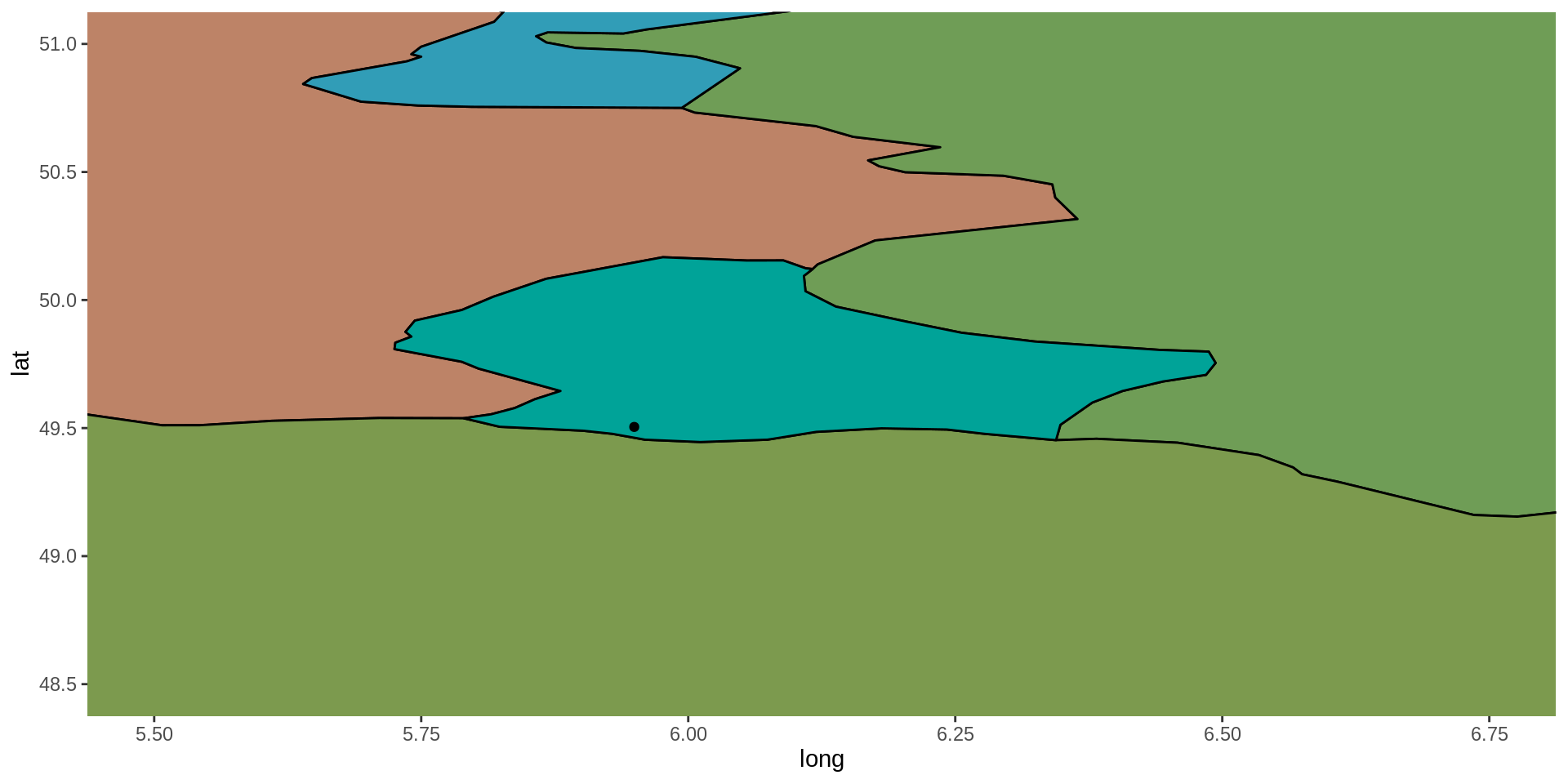

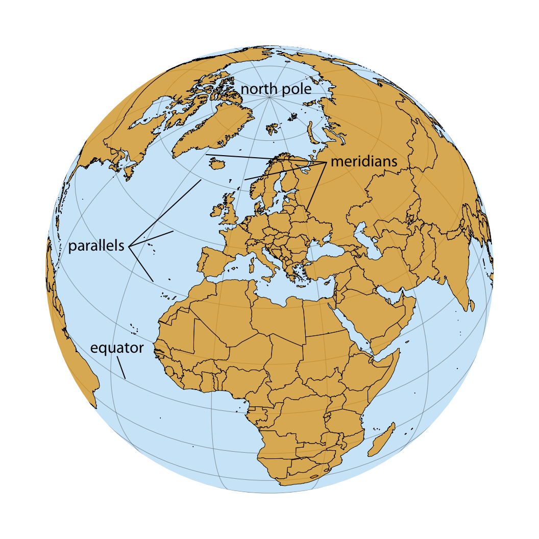
Projections

Why project?

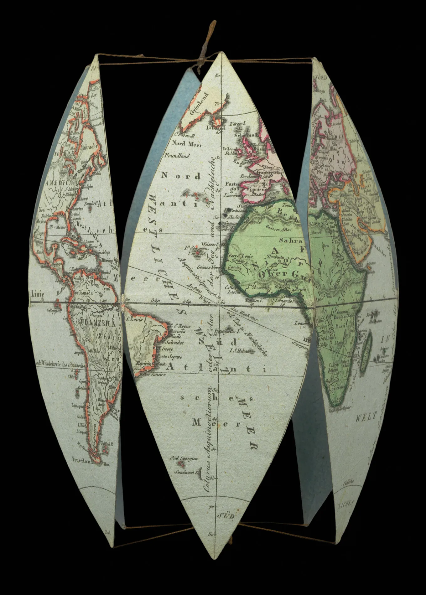
Parallels (latitude) and meridians (longitude)

Claus O. Wilke on projections.

There are many ways to project onto a 2D plane

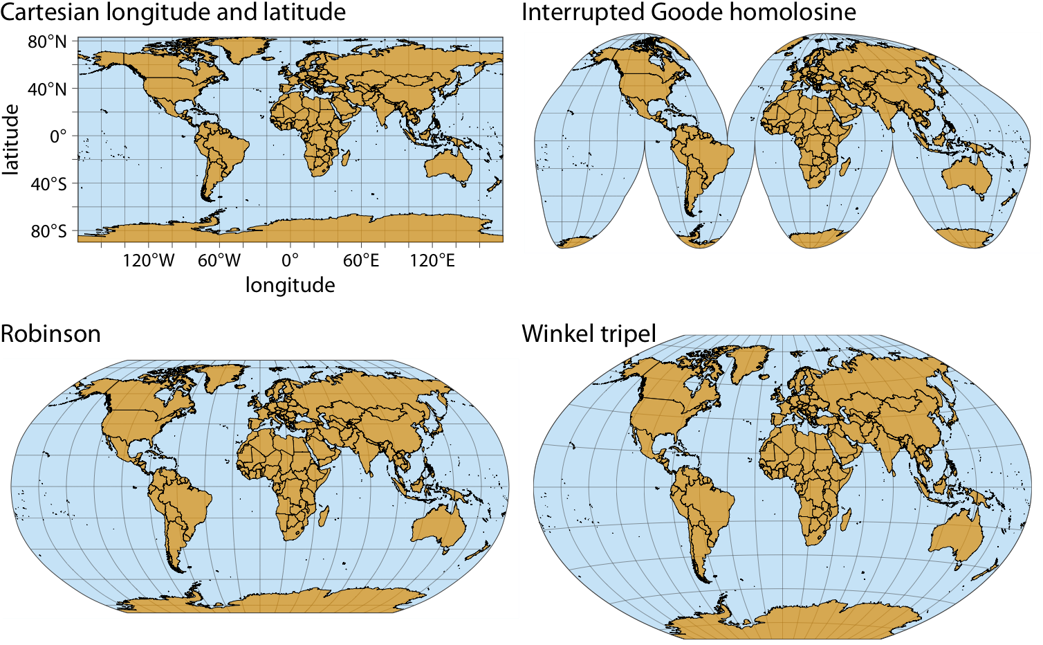
and many more in major families like

Cylindrical (e.g., Mercator, Cartesian/Plate Carrée)
Pseudocylindrical (e.g., Goode Homolosine, Robinson)
Conic
Planar
Modified/Compromised (e.g., Winkel triple)
Specialized

There are many ways to project onto a 2D plane

Mercator projection

Shapes are preserved, areas are severely distorted.

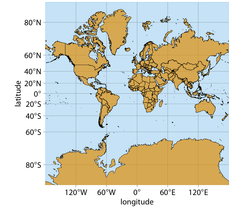
There are many ways to project onto a 2D plane

Mercator projection

Shapes are preserved, areas are severely distorted.

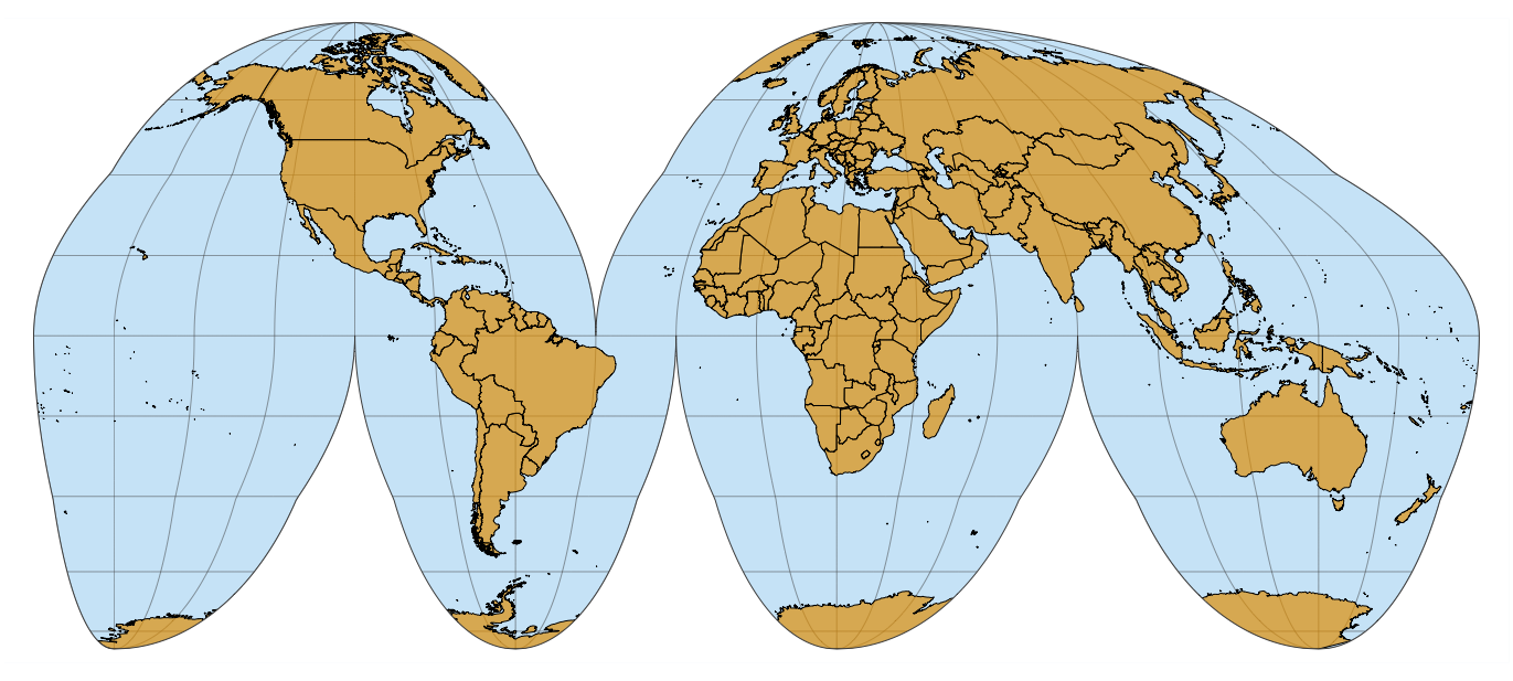
There are many ways to project onto a 2D plane

Goode homolosine

Areas are preserved, shapes are somewhat distorted

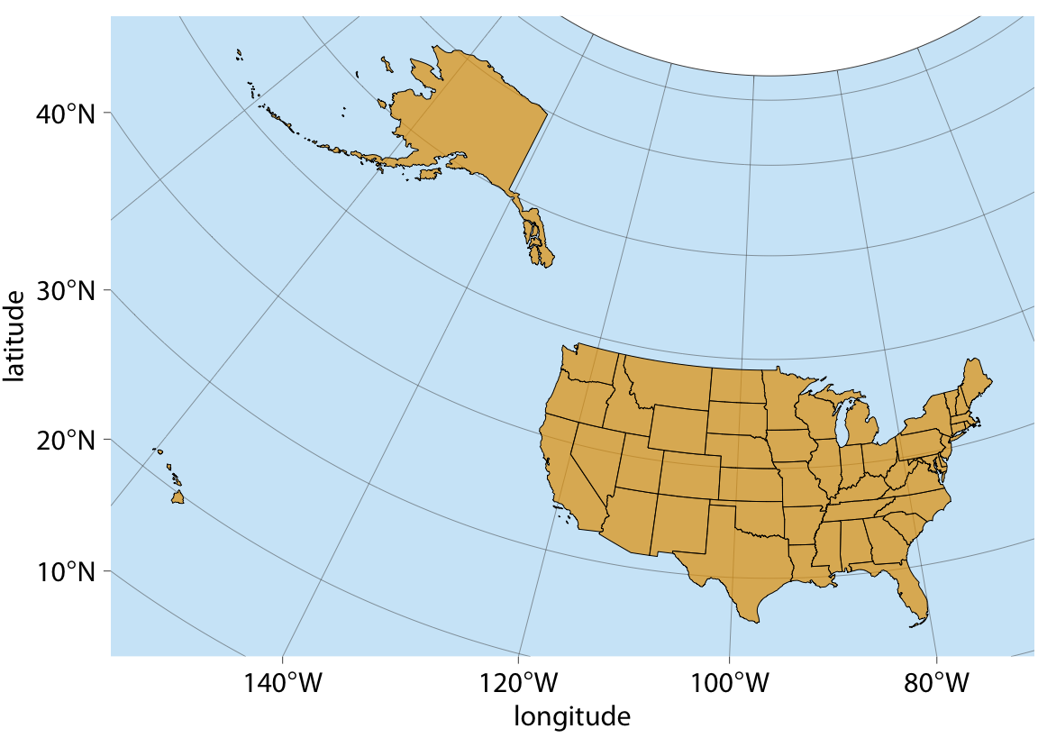
Projecting the US

Note

Alaska, Hawaii, and the lower 48 are far apart; difficult to show on one map

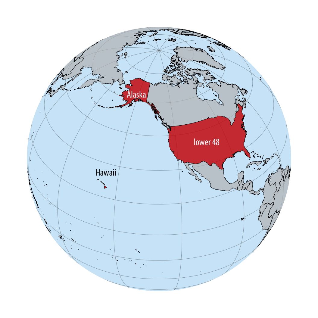
Projecting the US

A fair, area-preserving projection

Simple features - `sf`

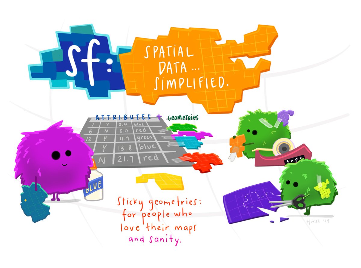
The sf package: Simple Features in R

Simple features in R

#euro_map <- world[world$continent == "Europe", ] # From R's `maps` package
euro_map <- rnaturalearth::ne_countries(scale = 110, 
                                        returnclass = 'sf', 
                                        continent = "Europe")

euro_map

Simple feature collection with 39 features and 168 fields
Geometry type: MULTIPOLYGON
Dimension:     XY
Bounding box:  xmin: -180 ymin: 2.053389 xmax: 180 ymax: 81.2504
Geodetic CRS:  WGS 84
First 10 features:
         featurecla scalerank labelrank sovereignt sov_a3 adm0_dif level
19  Admin-0 country         1         2     Russia    RUS        0     2
22  Admin-0 country         1         3     Norway    NOR        0     2
44  Admin-0 country         1         2     France    FR1        1     2
111 Admin-0 country         1         3     Sweden    SWE        0     2
112 Admin-0 country         1         4    Belarus    BLR        0     2
113 Admin-0 country         1         3    Ukraine    UKR        0     2
114 Admin-0 country         1         3     Poland    POL        0     2
115 Admin-0 country         1         4    Austria    AUT        0     2
116 Admin-0 country         1         5    Hungary    HUN        0     2
117 Admin-0 country         1         6    Moldova    MDA        0     2
                 type  tlc   admin adm0_a3 geou_dif geounit gu_a3 su_dif
19  Sovereign country    1  Russia     RUS        0  Russia   RUS      0
22  Sovereign country <NA>  Norway     NOR        0  Norway   NOR      0
44            Country    1  France     FRA        0  France   FRA      0
111 Sovereign country    1  Sweden     SWE        0  Sweden   SWE      0
112 Sovereign country    1 Belarus     BLR        0 Belarus   BLR      0
113 Sovereign country    1 Ukraine     UKR        0 Ukraine   UKR      0
114 Sovereign country    1  Poland     POL        0  Poland   POL      0
115 Sovereign country    1 Austria     AUT        0 Austria   AUT      0
116 Sovereign country    1 Hungary     HUN        0 Hungary   HUN      0
117 Sovereign country    1 Moldova     MDA        0 Moldova   MDA      0
    subunit su_a3 brk_diff    name          name_long brk_a3 brk_name brk_group
19   Russia   RUS        0  Russia Russian Federation    RUS   Russia      <NA>
22   Norway   NOR        0  Norway             Norway    NOR   Norway      <NA>
44   France   FRA        0  France             France    FRA   France      <NA>
111  Sweden   SWE        0  Sweden             Sweden    SWE   Sweden      <NA>
112 Belarus   BLR        0 Belarus            Belarus    BLR  Belarus      <NA>
113 Ukraine   UKR        0 Ukraine            Ukraine    UKR  Ukraine      <NA>
114  Poland   POL        0  Poland             Poland    POL   Poland      <NA>
115 Austria   AUT        0 Austria            Austria    AUT  Austria      <NA>
116 Hungary   HUN        0 Hungary            Hungary    HUN  Hungary      <NA>
117 Moldova   MDA        0 Moldova            Moldova    MDA  Moldova      <NA>
    abbrev postal           formal_en formal_fr name_ciawf note_adm0 note_brk
19    Rus.    RUS  Russian Federation      <NA>     Russia      <NA>     <NA>
22    Nor.      N   Kingdom of Norway      <NA>     Norway      <NA>     <NA>
44     Fr.      F     French Republic      <NA>     France      <NA>     <NA>
111   Swe.      S   Kingdom of Sweden      <NA>     Sweden      <NA>     <NA>
112  Bela.     BY Republic of Belarus      <NA>    Belarus      <NA>     <NA>
113   Ukr.     UA             Ukraine      <NA>    Ukraine      <NA>     <NA>
114   Pol.     PL  Republic of Poland      <NA>     Poland      <NA>     <NA>
115  Aust.      A Republic of Austria      <NA>    Austria      <NA>     <NA>
116   Hun.     HU Republic of Hungary      <NA>    Hungary      <NA>     <NA>
117   Mda.     MD Republic of Moldova      <NA>    Moldova      <NA>     <NA>
             name_sort name_alt mapcolor7 mapcolor8 mapcolor9 mapcolor13
19  Russian Federation     <NA>         2         5         7          7
22              Norway     <NA>         5         3         8         12
44              France     <NA>         7         5         9         11
111             Sweden     <NA>         1         4         2          4
112            Belarus     <NA>         1         1         5         11
113            Ukraine     <NA>         5         1         6          3
114             Poland     <NA>         3         7         1          2
115            Austria     <NA>         3         1         3          4
116            Hungary     <NA>         4         6         1          5
117            Moldova     <NA>         3         5         4         12
      pop_est pop_rank pop_year  gdp_md gdp_year                    economy
19  144373535       17     2019 1699876     2019   3. Emerging region: BRIC
22    5347896       13     2019  403336     2019 2. Developed region: nonG7
44   67059887       16     2019 2715518     2019    1. Developed region: G7
111  10285453       14     2019  530883     2019 2. Developed region: nonG7
112   9466856       13     2019   63080     2019       6. Developing region
113  44385155       15     2019  153781     2019       6. Developing region
114  37970874       15     2019  595858     2019 2. Developed region: nonG7
115   8877067       13     2019  445075     2019 2. Developed region: nonG7
116   9769949       13     2019  163469     2019 2. Developed region: nonG7
117   2657637       12     2019   11968     2019       6. Developing region
                income_grp fips_10 iso_a2 iso_a2_eh iso_a3 iso_a3_eh iso_n3
19  3. Upper middle income      RS     RU        RU    RUS       RUS    643
22    1. High income: OECD     -99    -99        NO    -99       NOR    -99
44    1. High income: OECD      FR    -99        FR    -99       FRA    -99
111   1. High income: OECD      SW     SE        SE    SWE       SWE    752
112 3. Upper middle income      BO     BY        BY    BLR       BLR    112
113 4. Lower middle income      UP     UA        UA    UKR       UKR    804
114   1. High income: OECD      PL     PL        PL    POL       POL    616
115   1. High income: OECD      AU     AT        AT    AUT       AUT    040
116   1. High income: OECD      HU     HU        HU    HUN       HUN    348
117 4. Lower middle income      MD     MD        MD    MDA       MDA    498
    iso_n3_eh un_a3 wb_a2 wb_a3   woe_id woe_id_eh
19        643   643    RU   RUS 23424936  23424936
22        578   -99   -99   -99      -90  23424910
44        250   250    FR   FRA      -90  23424819
111       752   752    SE   SWE 23424954  23424954
112       112   112    BY   BLR 23424765  23424765
113       804   804    UA   UKR 23424976  23424976
114       616   616    PL   POL 23424923  23424923
115       040   040    AT   AUT 23424750  23424750
116       348   348    HU   HUN 23424844  23424844
117       498   498    MD   MDA 23424885  23424885
                                                               woe_note
19                                           Exact WOE match as country
22  Does not include Svalbard, Jan Mayen, or Bouvet Islands (28289410).
44                Includes only Metropolitan France (including Corsica)
111                                          Exact WOE match as country
112                                          Exact WOE match as country
113                                          Exact WOE match as country
114                                          Exact WOE match as country
115                                          Exact WOE match as country
116                                          Exact WOE match as country
117                                          Exact WOE match as country
    adm0_iso adm0_diff adm0_tlc adm0_a3_us adm0_a3_fr adm0_a3_ru adm0_a3_es
19       RUS      <NA>      RUS        RUS        RUS        RUS        RUS
22       NOR      <NA>      NOR        NOR        NOR        NOR        NOR
44       FRA      <NA>      FRA        FRA        FRA        FRA        FRA
111      SWE      <NA>      SWE        SWE        SWE        SWE        SWE
112      BLR      <NA>      BLR        BLR        BLR        BLR        BLR
113      UKR      <NA>      UKR        UKR        UKR        UKR        UKR
114      POL      <NA>      POL        POL        POL        POL        POL
115      AUT      <NA>      AUT        AUT        AUT        AUT        AUT
116      HUN      <NA>      HUN        HUN        HUN        HUN        HUN
117      MDA      <NA>      MDA        MDA        MDA        MDA        MDA
    adm0_a3_cn adm0_a3_tw adm0_a3_in adm0_a3_np adm0_a3_pk adm0_a3_de
19         RUS        RUS        RUS        RUS        RUS        RUS
22         NOR        NOR        NOR        NOR        NOR        NOR
44         FRA        FRA        FRA        FRA        FRA        FRA
111        SWE        SWE        SWE        SWE        SWE        SWE
112        BLR        BLR        BLR        BLR        BLR        BLR
113        UKR        UKR        UKR        UKR        UKR        UKR
114        POL        POL        POL        POL        POL        POL
115        AUT        AUT        AUT        AUT        AUT        AUT
116        HUN        HUN        HUN        HUN        HUN        HUN
117        MDA        MDA        MDA        MDA        MDA        MDA
    adm0_a3_gb adm0_a3_br adm0_a3_il adm0_a3_ps adm0_a3_sa adm0_a3_eg
19         RUS        RUS        RUS        RUS        RUS        RUS
22         NOR        NOR        NOR        NOR        NOR        NOR
44         FRA        FRA        FRA        FRA        FRA        FRA
111        SWE        SWE        SWE        SWE        SWE        SWE
112        BLR        BLR        BLR        BLR        BLR        BLR
113        UKR        UKR        UKR        UKR        UKR        UKR
114        POL        POL        POL        POL        POL        POL
115        AUT        AUT        AUT        AUT        AUT        AUT
116        HUN        HUN        HUN        HUN        HUN        HUN
117        MDA        MDA        MDA        MDA        MDA        MDA
    adm0_a3_ma adm0_a3_pt adm0_a3_ar adm0_a3_jp adm0_a3_ko adm0_a3_vn
19         RUS        RUS        RUS        RUS        RUS        RUS
22         NOR        NOR        NOR        NOR        NOR        NOR
44         FRA        FRA        FRA        FRA        FRA        FRA
111        SWE        SWE        SWE        SWE        SWE        SWE
112        BLR        BLR        BLR        BLR        BLR        BLR
113        UKR        UKR        UKR        UKR        UKR        UKR
114        POL        POL        POL        POL        POL        POL
115        AUT        AUT        AUT        AUT        AUT        AUT
116        HUN        HUN        HUN        HUN        HUN        HUN
117        MDA        MDA        MDA        MDA        MDA        MDA
    adm0_a3_tr adm0_a3_id adm0_a3_pl adm0_a3_gr adm0_a3_it adm0_a3_nl
19         RUS        RUS        RUS        RUS        RUS        RUS
22         NOR        NOR        NOR        NOR        NOR        NOR
44         FRA        FRA        FRA        FRA        FRA        FRA
111        SWE        SWE        SWE        SWE        SWE        SWE
112        BLR        BLR        BLR        BLR        BLR        BLR
113        UKR        UKR        UKR        UKR        UKR        UKR
114        POL        POL        POL        POL        POL        POL
115        AUT        AUT        AUT        AUT        AUT        AUT
116        HUN        HUN        HUN        HUN        HUN        HUN
117        MDA        MDA        MDA        MDA        MDA        MDA
    adm0_a3_se adm0_a3_bd adm0_a3_ua adm0_a3_un adm0_a3_wb continent region_un
19         RUS        RUS        RUS        -99        -99    Europe    Europe
22         NOR        NOR        NOR        -99        -99    Europe    Europe
44         FRA        FRA        FRA        -99        -99    Europe    Europe
111        SWE        SWE        SWE        -99        -99    Europe    Europe
112        BLR        BLR        BLR        -99        -99    Europe    Europe
113        UKR        UKR        UKR        -99        -99    Europe    Europe
114        POL        POL        POL        -99        -99    Europe    Europe
115        AUT        AUT        AUT        -99        -99    Europe    Europe
116        HUN        HUN        HUN        -99        -99    Europe    Europe
117        MDA        MDA        MDA        -99        -99    Europe    Europe
          subregion             region_wb name_len long_len abbrev_len tiny
19   Eastern Europe Europe & Central Asia        6       18          4  -99
22  Northern Europe Europe & Central Asia        6        6          4  -99
44   Western Europe Europe & Central Asia        6        6          3  -99
111 Northern Europe Europe & Central Asia        6        6          4  -99
112  Eastern Europe Europe & Central Asia        7        7          5  -99
113  Eastern Europe Europe & Central Asia        7        7          4  -99
114  Eastern Europe Europe & Central Asia        6        6          4  -99
115  Western Europe Europe & Central Asia        7        7          5  -99
116  Eastern Europe Europe & Central Asia        7        7          4  -99
117  Eastern Europe Europe & Central Asia        7        7          4  -99
    homepart min_zoom min_label max_label   label_x  label_y      ne_id
19         1        0       1.7       5.2 44.686469 58.24936 1159321201
22         1        0       3.0       7.0  9.679975 61.35709 1159321109
44         1        0       1.7       6.7  2.552275 46.69611 1159320637
111        1        0       2.0       7.0 19.017050 65.85918 1159321287
112        1        0       3.0       8.0 28.417701 53.82189 1159320427
113        1        0       2.7       7.0 32.140865 49.72474 1159321345
114        1        0       2.5       7.0 19.490468 51.99032 1159321179
115        1        0       3.0       8.0 14.130515 47.51886 1159320379
116        1        0       4.0       9.0 19.447867 47.08684 1159320841
117        1        0       5.0      10.0 28.487904 47.43500 1159321045
    wikidataid   name_ar name_bn         name_de name_en     name_es  name_fa
19        Q159     روسيا  রাশিয়া        Russland  Russia       Rusia    روسیه
22         Q20   النرويج   নরওয়ে        Norwegen  Norway     Noruega     نروژ
44        Q142     فرنسا   ফ্রান্স      Frankreich  France     Francia   فرانسه
111        Q34    السويد   সুইডেন        Schweden  Sweden      Suecia     سوئد
112       Q184 بيلاروسيا  বেলারুশ         Belarus Belarus Bielorrusia   بلاروس
113       Q212  أوكرانيا  ইউক্রেন         Ukraine Ukraine     Ucrania  اوکراین
114        Q36    بولندا পোল্যান্ড           Polen  Poland     Polonia   لهستان
115        Q40    النمسا অস্ট্রিয়া      Österreich Austria     Austria    اتریش
116        Q28     المجر হাঙ্গেরি          Ungarn Hungary     Hungría مجارستان
117       Q217   مولدوفا  মলদোভা Republik Moldau Moldova    Moldavia  مولداوی
        name_fr    name_el  name_he name_hi          name_hu  name_id
19       Russie      Ρωσία    רוסיה      रूस      Oroszország    Rusia
22      Norvège   Νορβηγία נורווגיה    नॉर्वे         Norvégia Norwegia
44       France     Γαλλία     צרפת   फ़्रान्स    Franciaország  Prancis
111       Suède    Σουηδία   שוודיה   स्वीडन       Svédország   Swedia
112 Biélorussie Λευκορωσία   בלארוס   बेलारूस Fehéroroszország  Belarus
113     Ukraine   Ουκρανία אוקראינה    युक्रेन          Ukrajna  Ukraina
114     Pologne    Πολωνία    פולין    पोलैंड    Lengyelország Polandia
115    Autriche    Αυστρία  אוסטריה ऑस्ट्रिया         Ausztria  Austria
116     Hongrie   Ουγγαρία  הונגריה    हंगरी     Magyarország Hongaria
117    Moldavie   Μολδαβία  מולדובה मॉल्डोवा          Moldova  Moldova
        name_it      name_ja    name_ko     name_nl  name_pl      name_pt
19       Russia       ロシア     러시아     Rusland    Rosja       Rússia
22     Norvegia   ノルウェー   노르웨이   Noorwegen Norwegia      Noruega
44      Francia     フランス     프랑스   Frankrijk  Francja       França
111      Svezia スウェーデン     스웨덴      Zweden  Szwecja       Suécia
112 Bielorussia   ベラルーシ   벨라루스 Wit-Rusland Białoruś Bielorrússia
113     Ucraina   ウクライナ 우크라이나    Oekraïne  Ukraina      Ucrânia
114     Polonia   ポーランド     폴란드       Polen   Polska      Polónia
115     Austria オーストリア 오스트리아  Oostenrijk  Austria      Áustria
116    Ungheria   ハンガリー     헝가리   Hongarije    Węgry      Hungria
117    Moldavia     モルドバ     몰도바    Moldavië Mołdawia     Moldávia
       name_ru   name_sv     name_tr  name_uk name_ur   name_vi  name_zh
19      Россия  Ryssland       Rusya    Росія     روس       Nga   俄罗斯
22    Норвегия     Norge      Norveç Норвегія   ناروے     Na Uy     挪威
44     Франция Frankrike      Fransa  Франція   فرانس      Pháp     法国
111     Швеция   Sverige       İsveç   Швеція   سویڈن Thụy Điển     瑞典
112 Белоруссия   Belarus Beyaz Rusya Білорусь بیلاروس   Belarus 白俄罗斯
113    Украина   Ukraina     Ukrayna  Україна  یوکرین   Ukraina   乌克兰
114     Польша     Polen     Polonya   Польща  پولینڈ    Ba Lan     波兰
115    Австрия Österrike   Avusturya  Австрія  آسٹریا        Áo   奥地利
116    Венгрия    Ungern  Macaristan Угорщина   ہنگری   Hungary   匈牙利
117   Молдавия Moldavien     Moldova  Молдова مالدووا   Moldova 摩尔多瓦
    name_zht      fclass_iso tlc_diff      fclass_tlc fclass_us fclass_fr
19    俄羅斯 Admin-0 country     <NA> Admin-0 country      <NA>      <NA>
22      挪威    Unrecognized     <NA>    Unrecognized      <NA>      <NA>
44      法國 Admin-0 country     <NA> Admin-0 country      <NA>      <NA>
111     瑞典 Admin-0 country     <NA> Admin-0 country      <NA>      <NA>
112 白俄羅斯 Admin-0 country     <NA> Admin-0 country      <NA>      <NA>
113   烏克蘭 Admin-0 country     <NA> Admin-0 country      <NA>      <NA>
114     波蘭 Admin-0 country     <NA> Admin-0 country      <NA>      <NA>
115   奧地利 Admin-0 country     <NA> Admin-0 country      <NA>      <NA>
116   匈牙利 Admin-0 country     <NA> Admin-0 country      <NA>      <NA>
117 摩爾多瓦 Admin-0 country     <NA> Admin-0 country      <NA>      <NA>
    fclass_ru fclass_es fclass_cn fclass_tw fclass_in fclass_np fclass_pk
19       <NA>      <NA>      <NA>      <NA>      <NA>      <NA>      <NA>
22       <NA>      <NA>      <NA>      <NA>      <NA>      <NA>      <NA>
44       <NA>      <NA>      <NA>      <NA>      <NA>      <NA>      <NA>
111      <NA>      <NA>      <NA>      <NA>      <NA>      <NA>      <NA>
112      <NA>      <NA>      <NA>      <NA>      <NA>      <NA>      <NA>
113      <NA>      <NA>      <NA>      <NA>      <NA>      <NA>      <NA>
114      <NA>      <NA>      <NA>      <NA>      <NA>      <NA>      <NA>
115      <NA>      <NA>      <NA>      <NA>      <NA>      <NA>      <NA>
116      <NA>      <NA>      <NA>      <NA>      <NA>      <NA>      <NA>
117      <NA>      <NA>      <NA>      <NA>      <NA>      <NA>      <NA>
    fclass_de fclass_gb fclass_br fclass_il fclass_ps fclass_sa fclass_eg
19       <NA>      <NA>      <NA>      <NA>      <NA>      <NA>      <NA>
22       <NA>      <NA>      <NA>      <NA>      <NA>      <NA>      <NA>
44       <NA>      <NA>      <NA>      <NA>      <NA>      <NA>      <NA>
111      <NA>      <NA>      <NA>      <NA>      <NA>      <NA>      <NA>
112      <NA>      <NA>      <NA>      <NA>      <NA>      <NA>      <NA>
113      <NA>      <NA>      <NA>      <NA>      <NA>      <NA>      <NA>
114      <NA>      <NA>      <NA>      <NA>      <NA>      <NA>      <NA>
115      <NA>      <NA>      <NA>      <NA>      <NA>      <NA>      <NA>
116      <NA>      <NA>      <NA>      <NA>      <NA>      <NA>      <NA>
117      <NA>      <NA>      <NA>      <NA>      <NA>      <NA>      <NA>
    fclass_ma fclass_pt fclass_ar fclass_jp fclass_ko fclass_vn fclass_tr
19       <NA>      <NA>      <NA>      <NA>      <NA>      <NA>      <NA>
22       <NA>      <NA>      <NA>      <NA>      <NA>      <NA>      <NA>
44       <NA>      <NA>      <NA>      <NA>      <NA>      <NA>      <NA>
111      <NA>      <NA>      <NA>      <NA>      <NA>      <NA>      <NA>
112      <NA>      <NA>      <NA>      <NA>      <NA>      <NA>      <NA>
113      <NA>      <NA>      <NA>      <NA>      <NA>      <NA>      <NA>
114      <NA>      <NA>      <NA>      <NA>      <NA>      <NA>      <NA>
115      <NA>      <NA>      <NA>      <NA>      <NA>      <NA>      <NA>
116      <NA>      <NA>      <NA>      <NA>      <NA>      <NA>      <NA>
117      <NA>      <NA>      <NA>      <NA>      <NA>      <NA>      <NA>
    fclass_id fclass_pl fclass_gr fclass_it fclass_nl fclass_se fclass_bd
19       <NA>      <NA>      <NA>      <NA>      <NA>      <NA>      <NA>
22       <NA>      <NA>      <NA>      <NA>      <NA>      <NA>      <NA>
44       <NA>      <NA>      <NA>      <NA>      <NA>      <NA>      <NA>
111      <NA>      <NA>      <NA>      <NA>      <NA>      <NA>      <NA>
112      <NA>      <NA>      <NA>      <NA>      <NA>      <NA>      <NA>
113      <NA>      <NA>      <NA>      <NA>      <NA>      <NA>      <NA>
114      <NA>      <NA>      <NA>      <NA>      <NA>      <NA>      <NA>
115      <NA>      <NA>      <NA>      <NA>      <NA>      <NA>      <NA>
116      <NA>      <NA>      <NA>      <NA>      <NA>      <NA>      <NA>
117      <NA>      <NA>      <NA>      <NA>      <NA>      <NA>      <NA>
    fclass_ua                       geometry
19       <NA> MULTIPOLYGON (((178.7253 71...
22       <NA> MULTIPOLYGON (((15.14282 79...
44       <NA> MULTIPOLYGON (((-51.6578 4....
111      <NA> MULTIPOLYGON (((11.02737 58...
112      <NA> MULTIPOLYGON (((28.17671 56...
113      <NA> MULTIPOLYGON (((31.78599 52...
114      <NA> MULTIPOLYGON (((23.48413 53...
115      <NA> MULTIPOLYGON (((16.97967 48...
116      <NA> MULTIPOLYGON (((22.08561 48...
117      <NA> MULTIPOLYGON (((26.61934 48...

Plotting Europe

Code

ggplot(euro_map) +  geom_sf()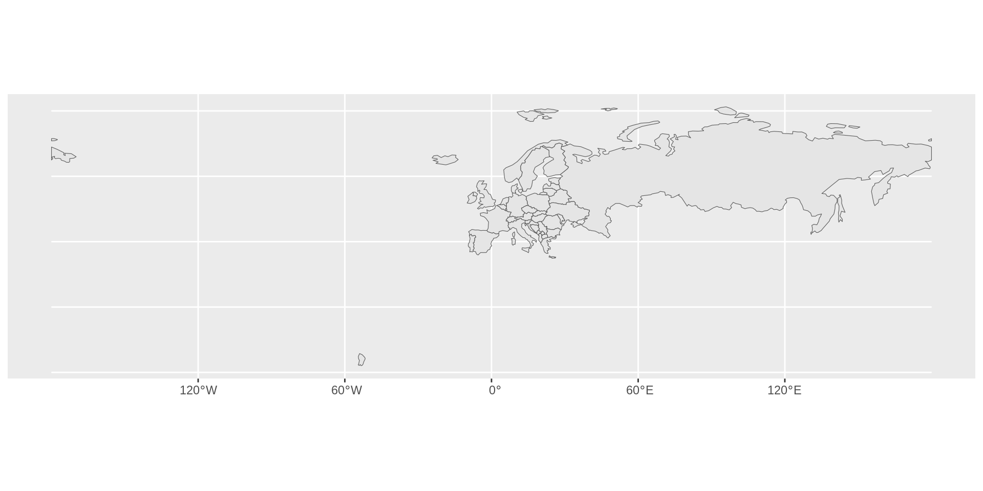

Plotting Europe geographically

Code

limits_x <- c(-25, 40)
limits_y <- c(32, 72.5)

euro_map |> 
  ggplot() +
  geom_sf() +
  coord_sf(xlim = limits_x,
           ylim = limits_y)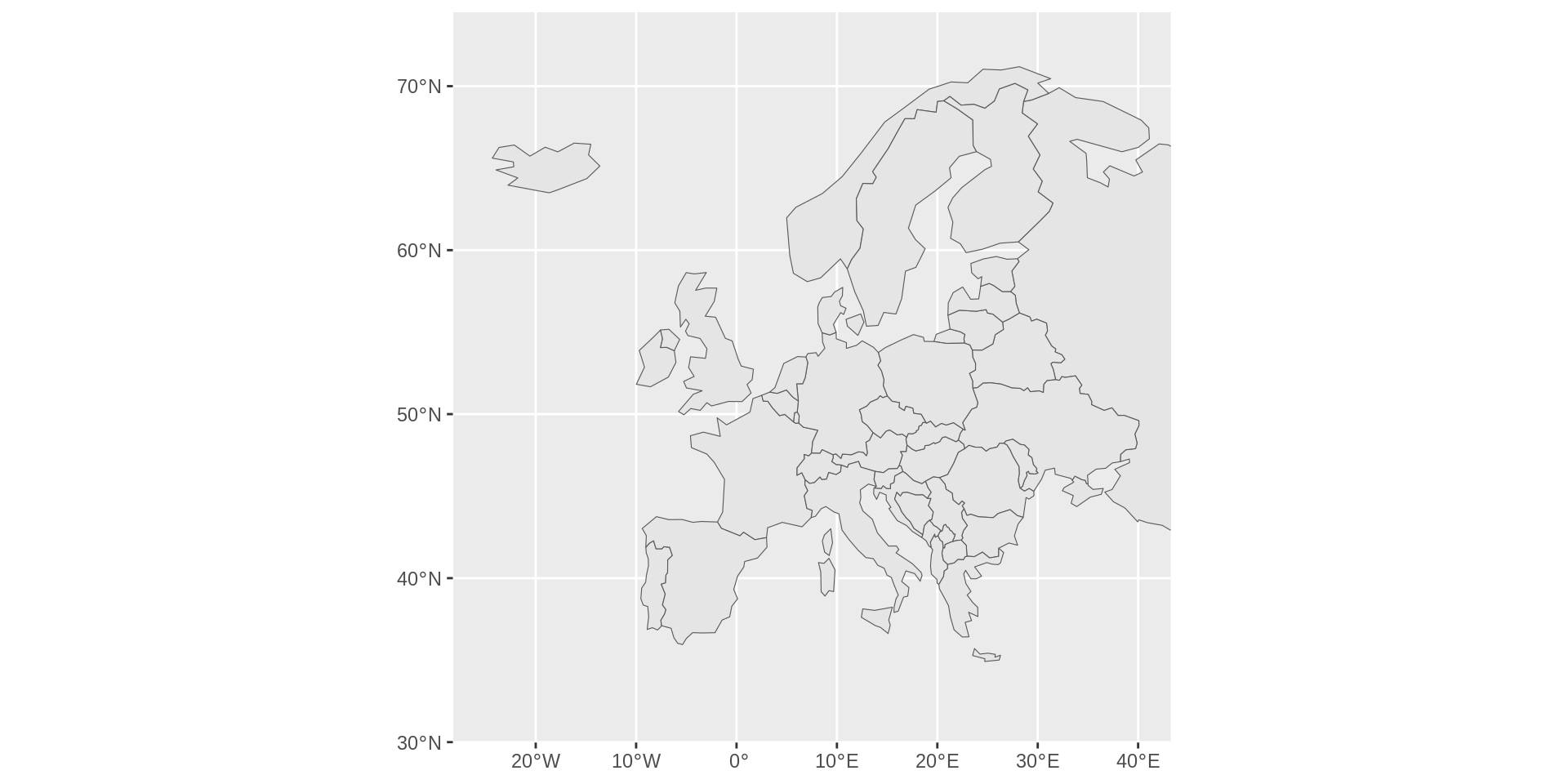

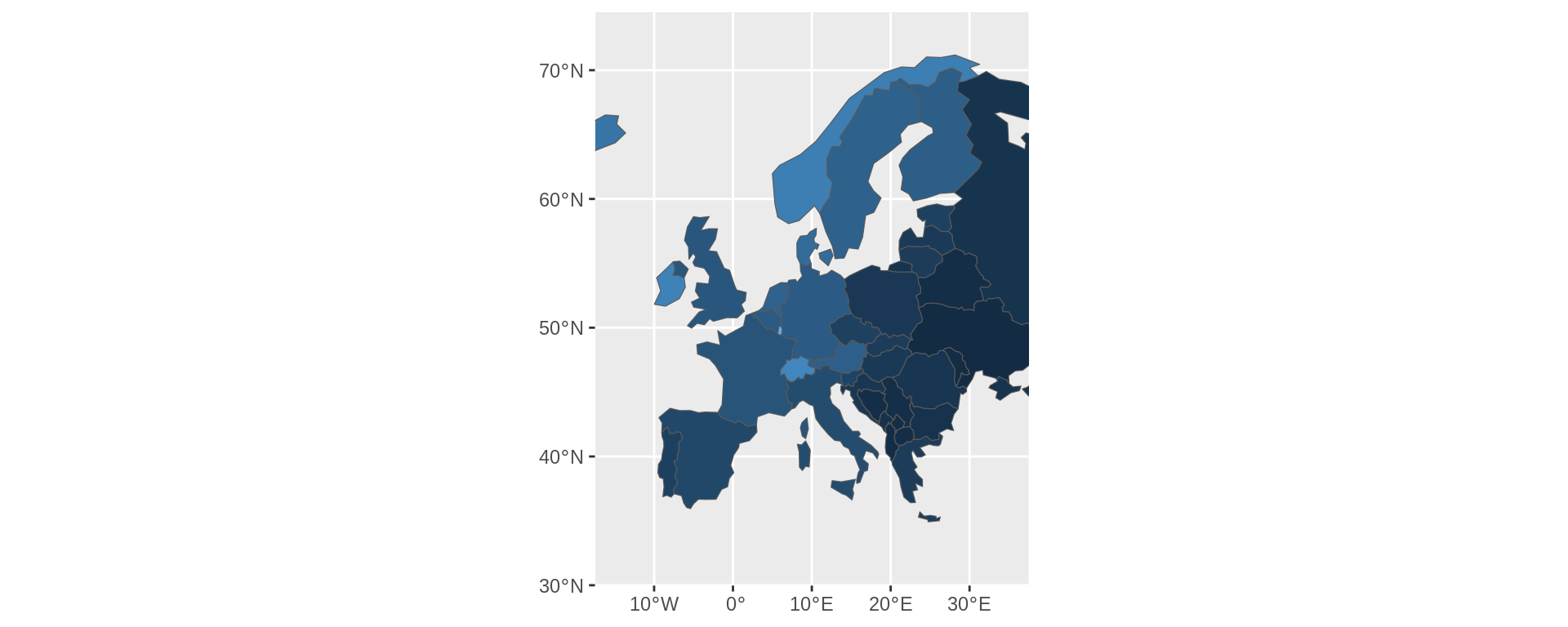
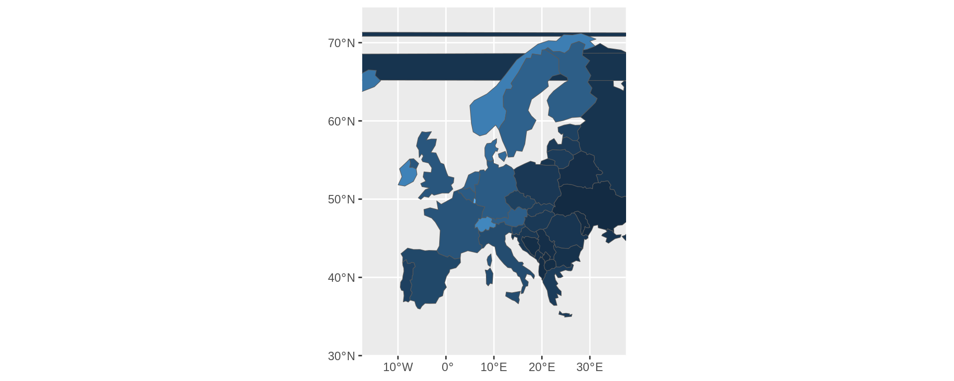
GDP per person in Europe

Code

euro_map |>
  ggplot() +
   geom_sf(aes(fill = gdp_md/pop_est)) + 
    coord_sf(xlim = limits_x,
           ylim = limits_y) +
  guides(fill = guide_legend(title = "GDP/Population")) +
  theme(legend.position = "bottom") +
  scale_fill_binned_sequential()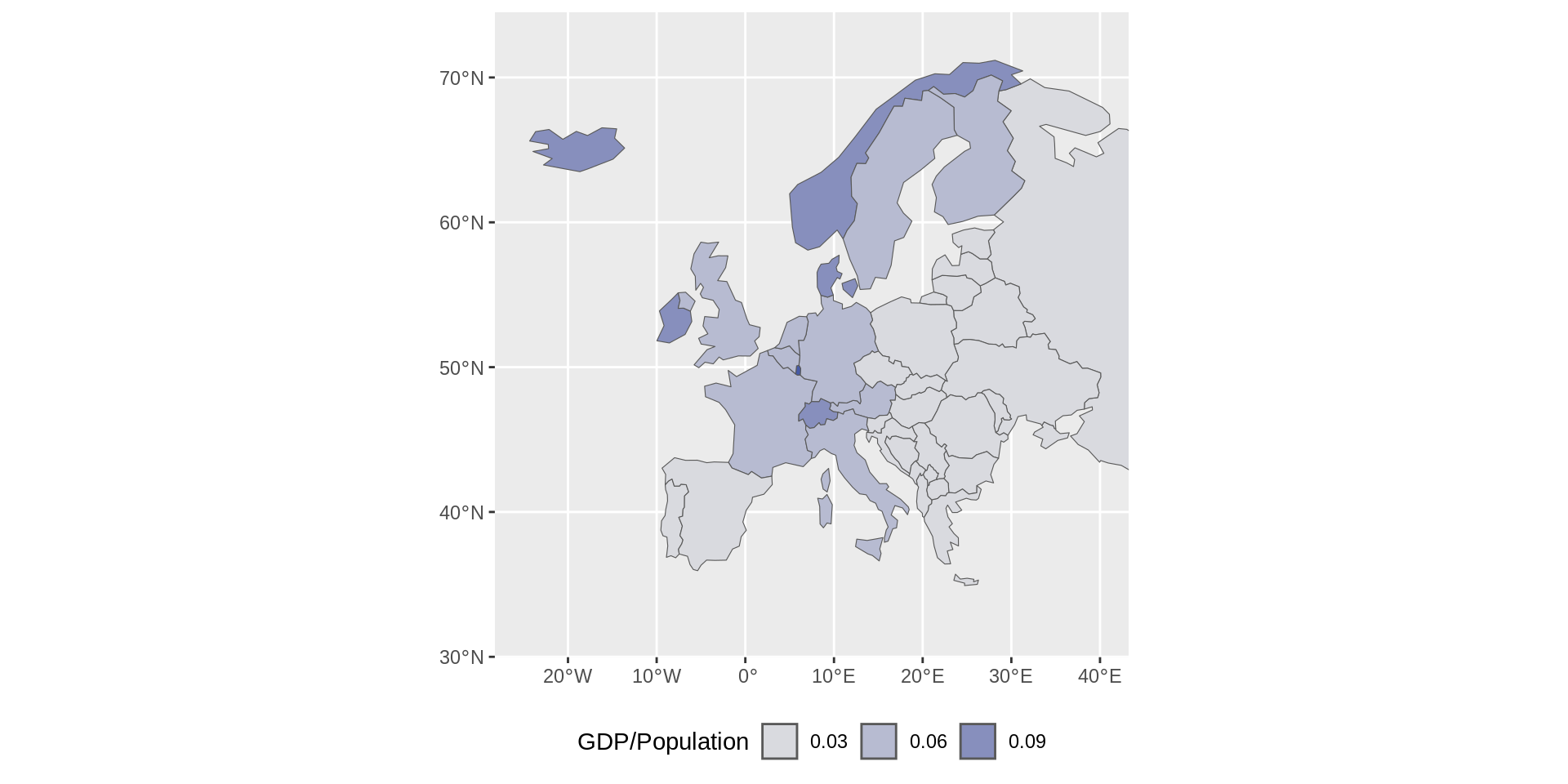

Your first choropleth!

from Ancient Greek χῶρος (khôros) ‘area, region’ and πλῆθος (plêthos) ‘multitude’) is a type of statistical thematic map that uses pseudocolor, meaning color corresponding with an aggregate summary of a geographic characteristic within spatial enumeration units, such as population density or per-capita income.

GDP per person in Europe - white borders

euro_map |>
  ggplot() +
  geom_sf(aes(fill = gdp_md/pop_est),
          colour = "white") + 
  coord_sf(xlim = limits_x,
           ylim = limits_y) +
  guides(fill = guide_legend(title = "GDP/Population"))+
  theme(legend.position = "bottom") +
  scale_fill_binned_sequential()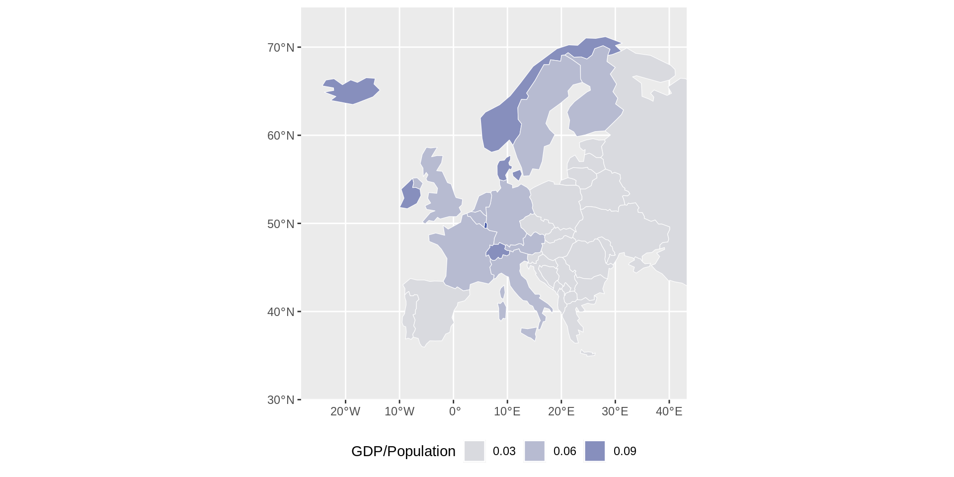

Select Luxembourg

euro_map |> 
   filter(name == "Luxembourg") |> 
   relocate(geometry)

Simple feature collection with 1 feature and 168 fields
Geometry type: MULTIPOLYGON
Dimension:     XY
Bounding box:  xmin: 5.674052 ymin: 49.44267 xmax: 6.242751 ymax: 50.12805
Geodetic CRS:  WGS 84
                        geometry      featurecla scalerank labelrank sovereignt
1 MULTIPOLYGON (((6.043073 50... Admin-0 country         1         6 Luxembourg
  sov_a3 adm0_dif level              type tlc      admin adm0_a3 geou_dif
1    LUX        0     2 Sovereign country   1 Luxembourg     LUX        0
     geounit gu_a3 su_dif    subunit su_a3 brk_diff       name  name_long
1 Luxembourg   LUX      0 Luxembourg   LUX        0 Luxembourg Luxembourg
  brk_a3   brk_name brk_group abbrev postal                 formal_en formal_fr
1    LUX Luxembourg      <NA>   Lux.      L Grand Duchy of Luxembourg      <NA>
  name_ciawf note_adm0 note_brk  name_sort name_alt mapcolor7 mapcolor8
1 Luxembourg      <NA>     <NA> Luxembourg     <NA>         1         7
  mapcolor9 mapcolor13 pop_est pop_rank pop_year gdp_md gdp_year
1         3          7  619896       11     2019  71104     2019
                     economy           income_grp fips_10 iso_a2 iso_a2_eh
1 2. Developed region: nonG7 1. High income: OECD      LU     LU        LU
  iso_a3 iso_a3_eh iso_n3 iso_n3_eh un_a3 wb_a2 wb_a3   woe_id woe_id_eh
1    LUX       LUX    442       442   442    LU   LUX 23424881  23424881
                    woe_note adm0_iso adm0_diff adm0_tlc adm0_a3_us adm0_a3_fr
1 Exact WOE match as country      LUX      <NA>      LUX        LUX        LUX
  adm0_a3_ru adm0_a3_es adm0_a3_cn adm0_a3_tw adm0_a3_in adm0_a3_np adm0_a3_pk
1        LUX        LUX        LUX        LUX        LUX        LUX        LUX
  adm0_a3_de adm0_a3_gb adm0_a3_br adm0_a3_il adm0_a3_ps adm0_a3_sa adm0_a3_eg
1        LUX        LUX        LUX        LUX        LUX        LUX        LUX
  adm0_a3_ma adm0_a3_pt adm0_a3_ar adm0_a3_jp adm0_a3_ko adm0_a3_vn adm0_a3_tr
1        LUX        LUX        LUX        LUX        LUX        LUX        LUX
  adm0_a3_id adm0_a3_pl adm0_a3_gr adm0_a3_it adm0_a3_nl adm0_a3_se adm0_a3_bd
1        LUX        LUX        LUX        LUX        LUX        LUX        LUX
  adm0_a3_ua adm0_a3_un adm0_a3_wb continent region_un      subregion
1        LUX        -99        -99    Europe    Europe Western Europe
              region_wb name_len long_len abbrev_len tiny homepart min_zoom
1 Europe & Central Asia       10       10          4    5        1        0
  min_label max_label label_x  label_y      ne_id wikidataid   name_ar  name_bn
1       5.7        10 6.07762 49.73373 1159321031        Q32 لوكسمبورغ লুক্সেমবুর্গ
    name_de    name_en    name_es    name_fa    name_fr      name_el   name_he
1 Luxemburg Luxembourg Luxemburgo لوکزامبورگ Luxembourg Λουξεμβούργο לוקסמבורג
  name_hi   name_hu    name_id     name_it        name_ja    name_ko   name_nl
1 लक्ज़मबर्ग Luxemburg Luksemburg Lussemburgo ルクセンブルク 룩셈부르크 Luxemburg
     name_pl    name_pt    name_ru   name_sv    name_tr    name_uk name_ur
1 Luksemburg Luxemburgo Люксембург Luxemburg Lüksemburg Люксембург لکسمبرگ
     name_vi name_zh name_zht      fclass_iso tlc_diff      fclass_tlc
1 Luxembourg  卢森堡   盧森堡 Admin-0 country     <NA> Admin-0 country
  fclass_us fclass_fr fclass_ru fclass_es fclass_cn fclass_tw fclass_in
1      <NA>      <NA>      <NA>      <NA>      <NA>      <NA>      <NA>
  fclass_np fclass_pk fclass_de fclass_gb fclass_br fclass_il fclass_ps
1      <NA>      <NA>      <NA>      <NA>      <NA>      <NA>      <NA>
  fclass_sa fclass_eg fclass_ma fclass_pt fclass_ar fclass_jp fclass_ko
1      <NA>      <NA>      <NA>      <NA>      <NA>      <NA>      <NA>
  fclass_vn fclass_tr fclass_id fclass_pl fclass_gr fclass_it fclass_nl
1      <NA>      <NA>      <NA>      <NA>      <NA>      <NA>      <NA>
  fclass_se fclass_bd fclass_ua
1      <NA>      <NA>      <NA>

#lux <-  world[world$name_long == "Luxembourg", ]

Plotting Luxembourg

ggplot(
euro_map |> 
   filter(name == "Luxembourg") |> 
   relocate(geometry)) + geom_sf()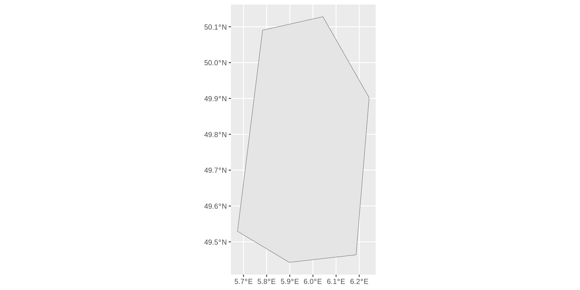

More resolution is needed

euro_map50 <- rnaturalearth::ne_countries(
  scale = 50, 
  type = 'map_units', 
  returnclass = 'sf')

euro_map50 |> filter(name == "Luxembourg") |> 
  ggplot() +
  geom_sf()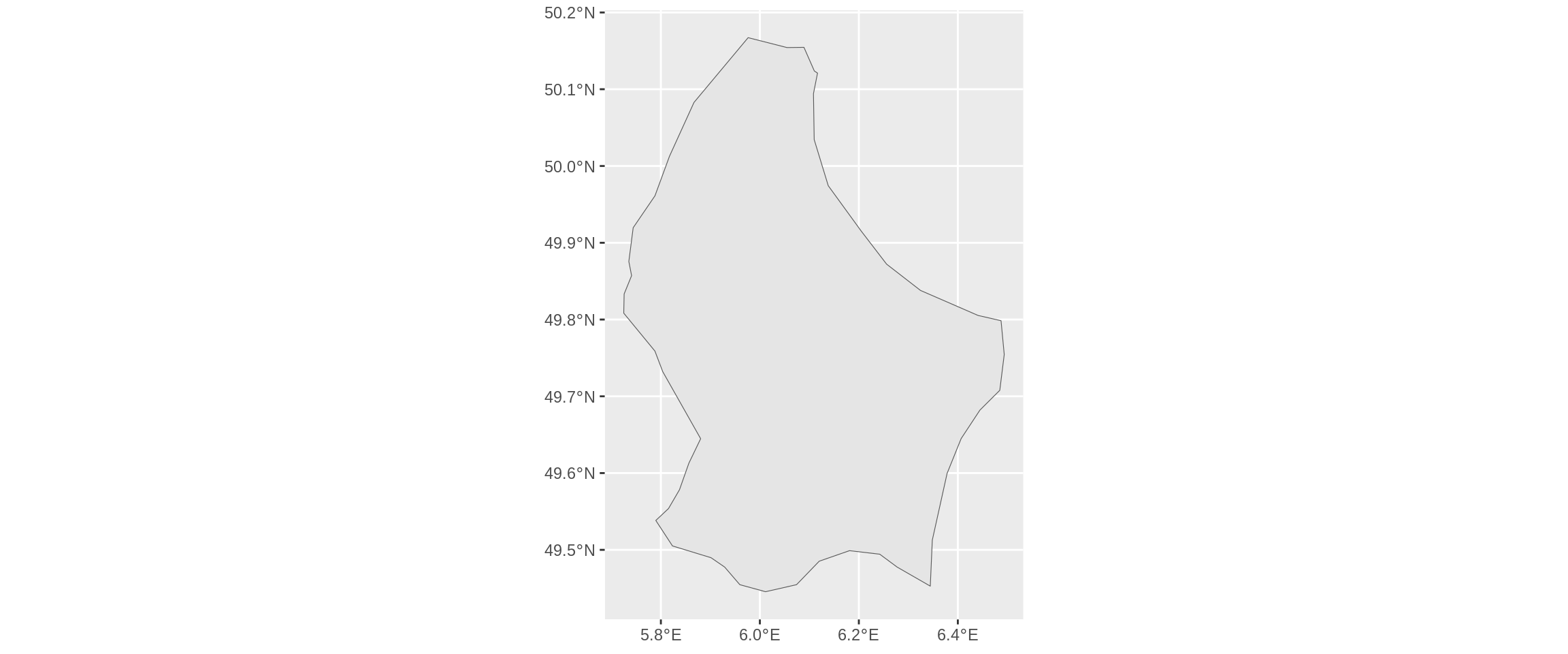

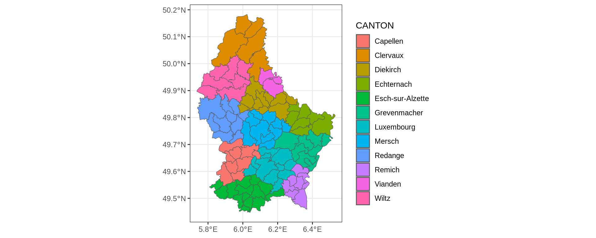
High-resolution maps from Shapefiles

f = system.file("shapes/world.gpkg", package = "spData")
world = read_sf(f)

lux_shp <- sf::st_read("data/LIMADM_COMMUNES.shp")

Reading layer `LIMADM_COMMUNES' from data source 
  `/builds/NZds3xjaf/0/uniluxembourg/lcsb/r-training/mads6/slides/data/LIMADM_COMMUNES.shp' 
  using driver `ESRI Shapefile'
Simple feature collection with 102 features and 4 fields
Geometry type: MULTIPOLYGON
Dimension:     XY
Bounding box:  xmin: 48930.25 ymin: 57015.29 xmax: 106113.8 ymax: 138759.2
Projected CRS: Luxembourg_1930_Gauss

ggplot(lux_shp) + 
  geom_sf(aes(fill = CANTON)) +
  theme_bw() -> lux_commune_map

lux_commune_map +
#  paletteer::scale_fill_paletteer_d("rtist::vangogh")
  scale_fill_discrete_qualitative(palette = "Dark 3")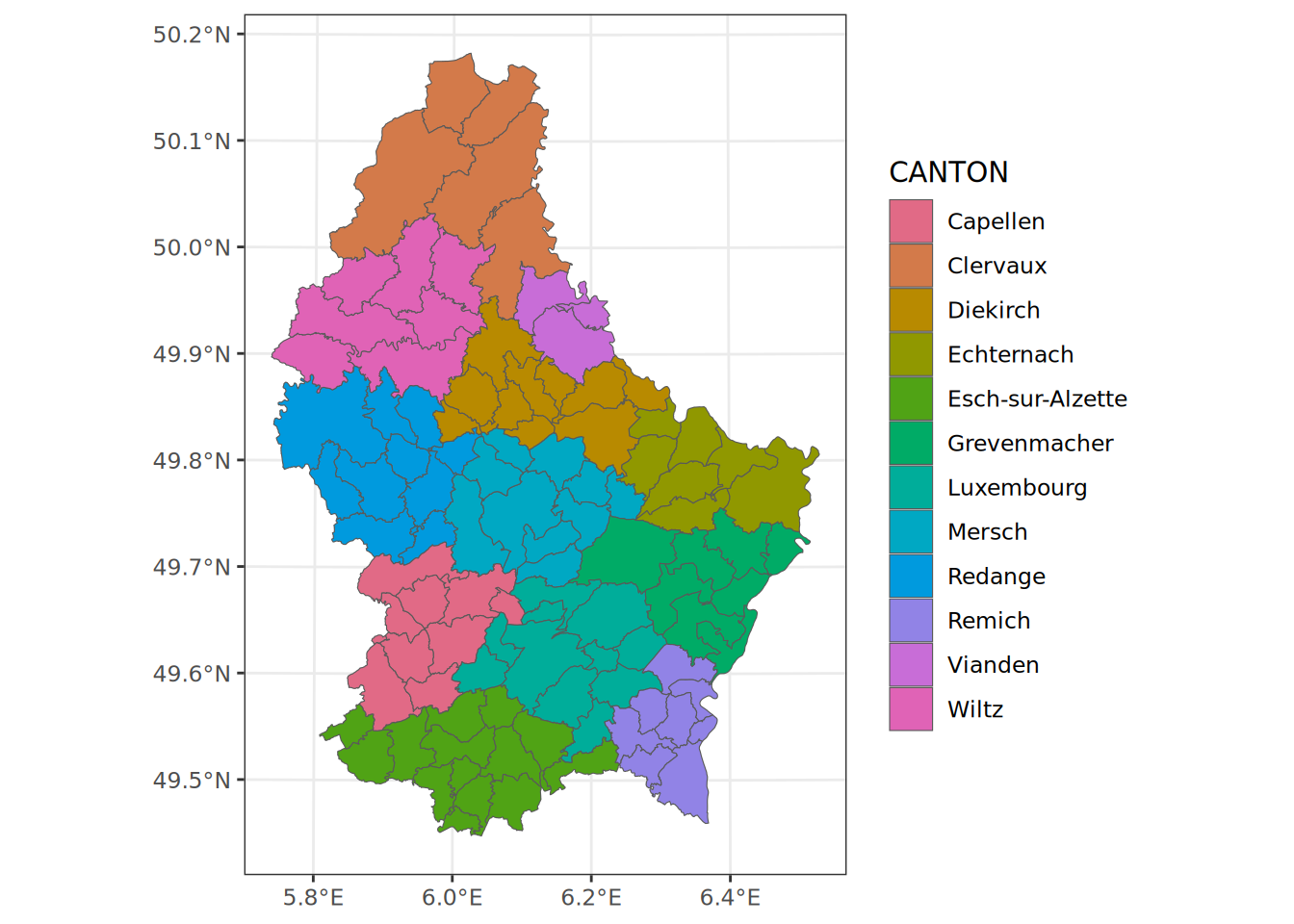

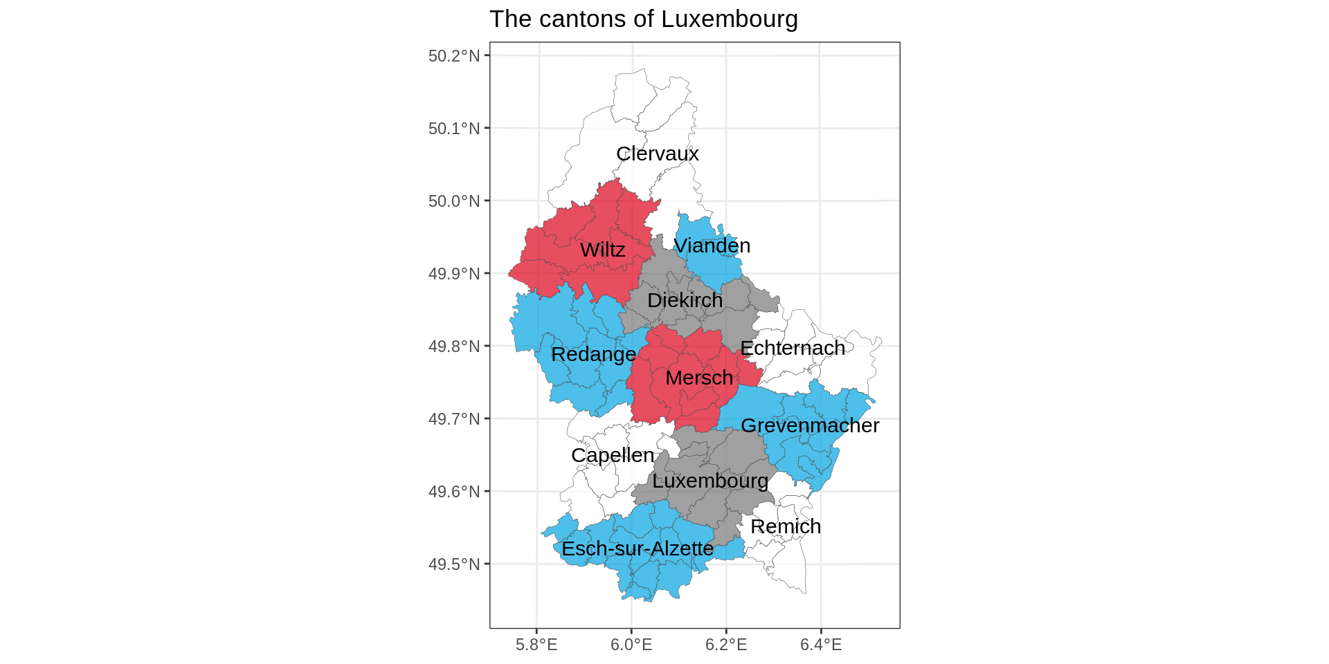
Four color theorem

Code

commune <- c(
  Redange = "#00A4E1",
  Grevenmacher = "#00A4E1",
  Luxembourg = "#777",
  Vianden = "#00A4E1",
  Mersch = "#DC021B",
  "Esch-sur-Alzette" = "#00A4E1",
  Wiltz = "#DC021B",
  Clervaux = "#FFF",
  Diekirch = "#777",
  Remich =  "#FFF",
  Capellen = "#FFF",
  Echternach = "#FFF"
)

lux_shp |> 
  group_by(CANTON) |> 
  mutate(n = row_number(),
    canton_label = if_else(n ==1, CANTON, ""),
    # centroid of each elements (county level)
    lon = st_coordinates(st_centroid(geometry))[,1],
    lat = st_coordinates(st_centroid(geometry))[,2],
    # median lon/lat of county centroids. It's a hack.
    med_lon = median(lon),
    med_lat = median(lat))  |> 
  ungroup() |> 
ggplot() + 
  geom_sf(aes(fill = CANTON) , 
          alpha = 0.7, 
          show.legend = FALSE, linewidth = 0.1) +
  theme_bw()  + scale_fill_manual(values = commune) +
  geom_text(aes(x = med_lon, y = med_lat, label = canton_label), size = 4) +
  # geom_sf_text does not take x, y
  labs(title = "The cantons of Luxembourg",
       x = NULL, 
       y = NULL)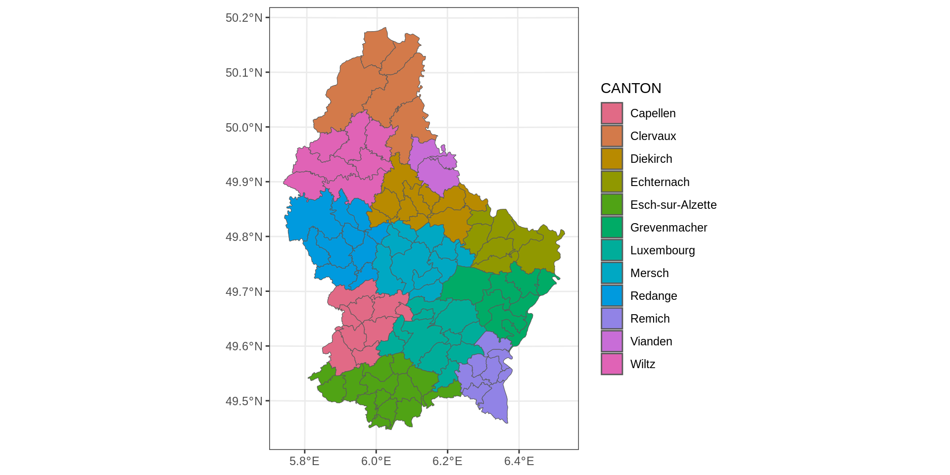

Transforming using the Coordinate Reference System (CRS)

CRS 4326

euro_map |> 
  ggplot() +
 geom_sf(aes(fill = gdp_md/pop_est)) + 
    coord_sf(xlim = c(-15, 35),
           ylim = c(32, 72.5), 
           crs = 4326) + # CRS!
  guides(fill = "none")

CRS 4181

euro_map |> 
  ggplot() +
 geom_sf(aes(fill = gdp_md/pop_est)) + 
    coord_sf(xlim = c(-15, 35),
           ylim = c(32, 72.5),
           crs = 4181) + # Different CRS!
  guides(fill = "none")

Luxembourg by different CRS

CRS 4326

lux_commune_map + coord_sf(crs = 4326)

CRS 4100

lux_commune_map + coord_sf(crs = 4100)

CRS transform needs to be applied to all spatial data

(ggplot(data = world) +
  geom_sf(mapping = aes(fill = continent)) +
  scale_fill_viridis_d(name = "Continent",
                      na.value = "grey50") +
  #theme(legend.position = "bottom") +
  coord_sf(crs = 3857) # CRS for Web Mercator projection
  -> continent_map)

We want to add our spot; just using coordinates will not work after transformations.

mno_1020

    long     lat
1 5.9479 49.5037

Web Mercator

+ coord_sf(crs = 3857):
De facto standard for online mapping services like Google Maps, OpenStreetMap, and Bing Maps.
Assumes spherical earth, hence computationally faster, which is relevant for web applications.

CRS transform needs to be applied to all spatial data

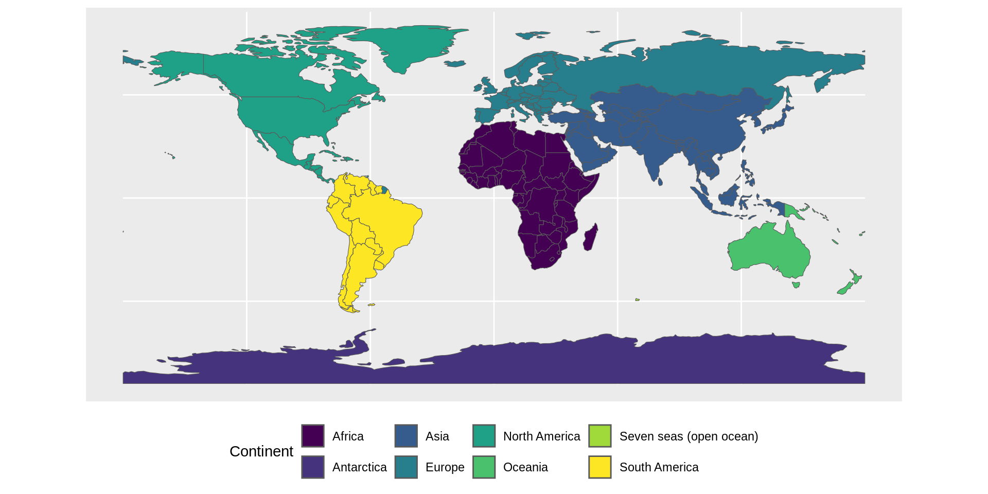
continent_map +
  geom_point(data = mno_1020,
             aes(x = long, y = lat),
             color = "red") +
    geom_label_repel(data = mno_1020,
                  aes(x = long, y = lat, label = "MNO"),
                  fill="black",
                  color = "white",
                  size = 3,
                  label.r = unit(0.25, "lines"), # rounded corners
                  label.size = 0.4, # border thickness
                  segment.color = "white",
                  segment.size = 0.7,
                  nudge_y = 0.3, # Keep label above
                  force=5 # Keep label further away
                  ) +
  theme(axis.title = element_blank()) # Needed as geom_point as labels.

Note

Latitude/longitude is WGS84 (EPSG:4326), i.e., standard GPS coordinates.
Does not fit with select CRS (Web Mercator, EPSG: 3857).
EPSG stands for European Petroleum Survey Group.

CRS transform needs to be applied to all spatial data

# Converting our position
mno_1020_sf <- st_as_sf(mno_1020, 
         coords = c("long", "lat"), 
         crs = 4326) %>%  # Specify it's in WGS84
  st_transform(crs = 3857)  # Transform to Web Mercator

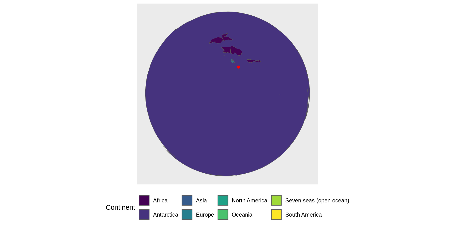
continent_map +
  geom_sf(data = mno_1020_sf, # New simple feature to be plotted
          color = "red") +
  coord_sf(crs = 3857) # Web Mercator. Specify CRS for entire plot!

CRS for Luxembourg

CRS2169
- Projected
- Flat coordinates in meters based on Transverse Mercator
- Current official CRS for Luxembourg (LUREF)
CRS4181
- Unprojected
- Spherical coordinates in degrees
- Historical system

Zoom in

continent_map +
  geom_sf(data = mno_1020_sf, # New simple feature to be plotted
          color = "red") +
  coord_sf(crs = 3857, # Web Mercator. Specify CRS for entire plot!
            xlim = c(5.5, 6.75),
            ylim = c(48.5, 51),
            default_crs = 4326)

Considerations

Make sure to think about scale.

And whether a simple zoom is actually the right way …

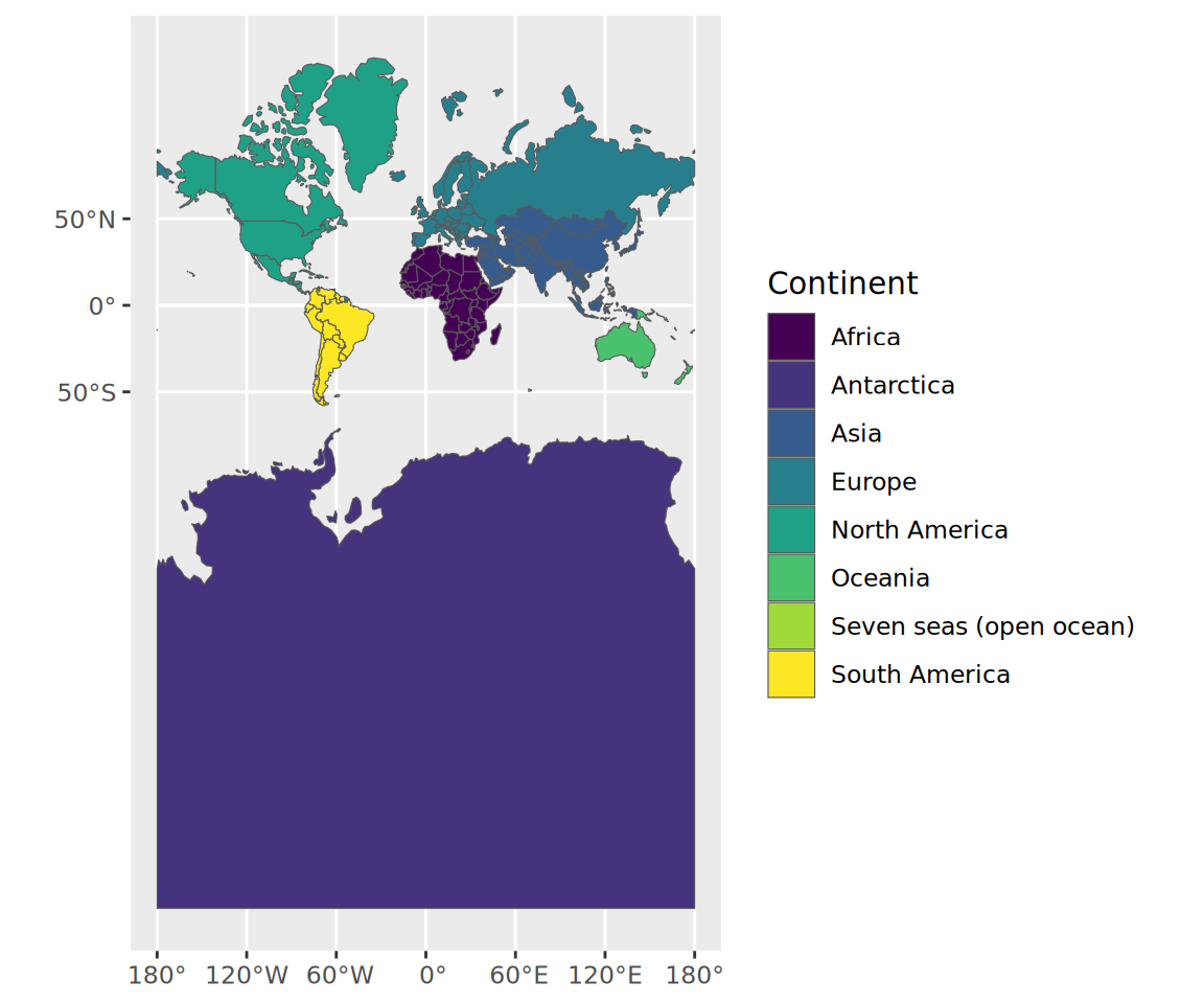
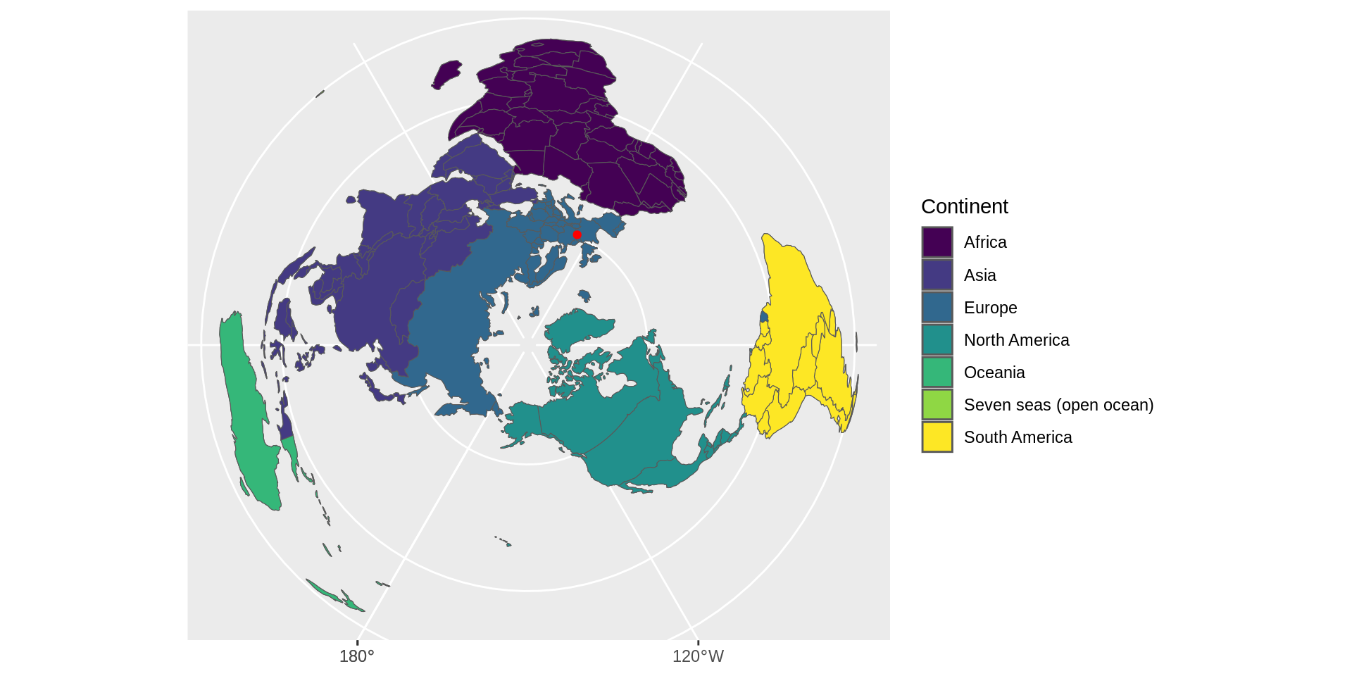
View from the pole

continent_map +
  # Converting our position
  geom_sf(data = mno_1020_sf, color = "red") +
  # rotating globe
  coord_sf(crs = 3572) # Make sure to specify CRS for entire plot

Removing Antarctica

world |> 
  filter(continent != "Antarctica") |> 
ggplot() +
  geom_sf() +
  geom_sf(mapping = aes(fill = continent)) +
  scale_fill_viridis_d(name = "Continent",
                      na.value = "grey50") +
  # Converting our position
  geom_sf(data = mno_1020_sf, color = "red") +
  # rotating globe
  coord_sf(crs = 3572)

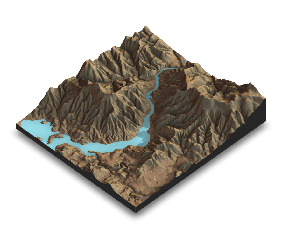
When 3D is ok

Going from this

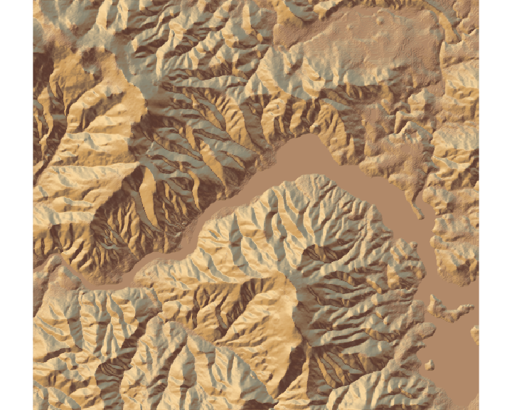The rayshader package allows to produce 2D and 3D data visualizations in R.

to this

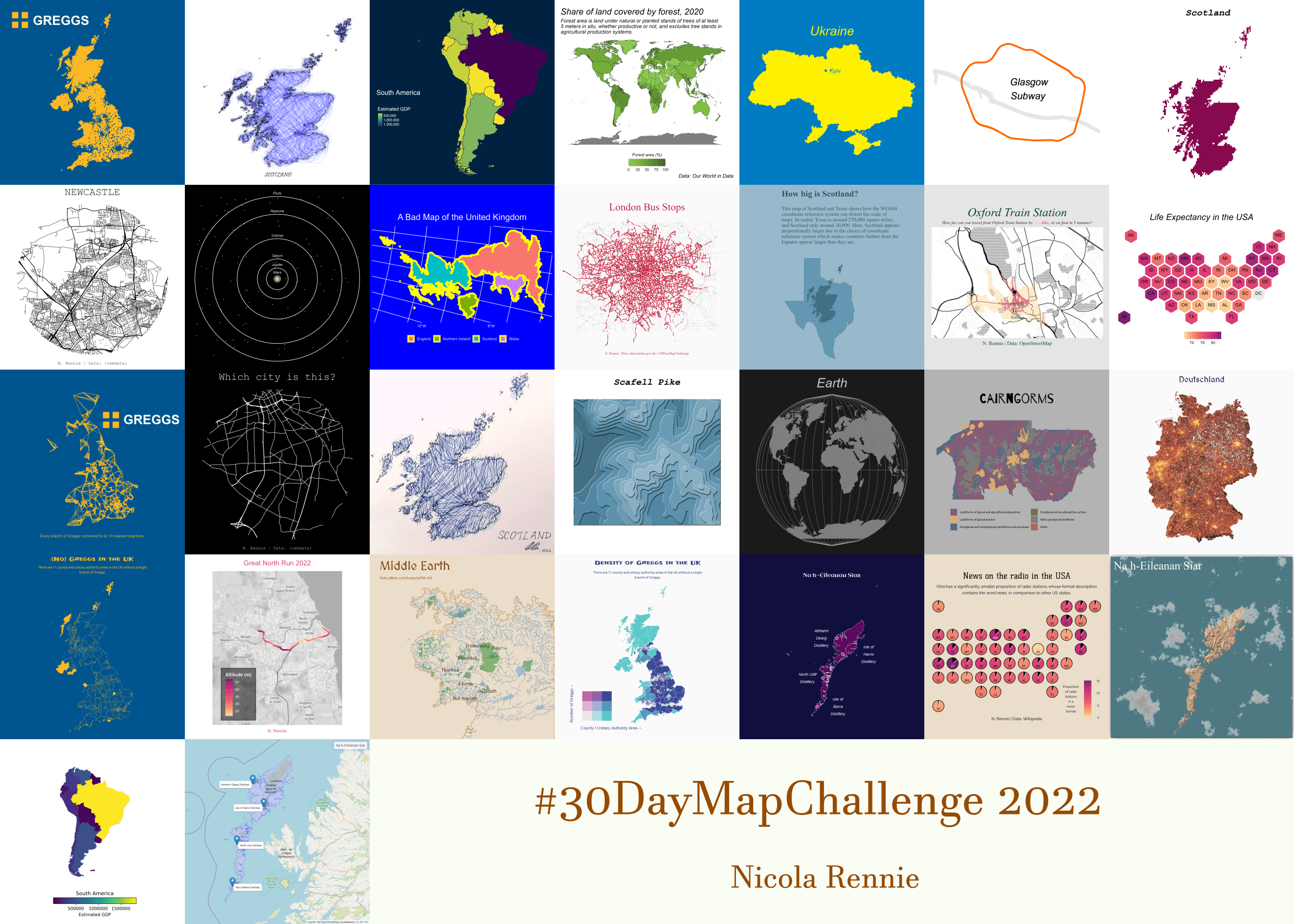
Want to hone your skills?

The 30 Day Map Challenge

30 Day Map Challenge repo
Typically takes place in November
An example from Nicola Rennie

Before we stop

We looked at

Basic maps in ggplot
Spatial features in sf
Data from the Natural Earth project in R
Importing Shapefiles for high-resolution maps
Using the Coordinate Reference System

Acknowledgements

Claus O. Wilke

Geographical data

Introduction

Maps

Learning objectives

Material

Basic maps

But first: why do maps matter?

Basic map data in R

Basics from maps

Basic maps with ggplot

Using maps

Basic maps with ggplot

ggplot knows the world

… which we can easily visualise

Basic maps with ggplot

ggplot knows the world

… which we can easily visualise if groups are respected

geom_polygon() give us countries

geom_map()

Zooming in on Luxembourg

Projections

Why project?

Parallels (latitude) and meridians (longitude)

There are many ways to project onto a 2D plane

and many more in major families like

There are many ways to project onto a 2D plane

Mercator projection

There are many ways to project onto a 2D plane

Mercator projection

There are many ways to project onto a 2D plane

Goode homolosine

Projecting the US

Projecting the US

Simple features - sf

The sf package: Simple Features in R

Simple features in R

Plotting Europe

Plotting Europe geographically

GDP per person in Europe

Your first choropleth!

GDP per person in Europe - white borders

Select Luxembourg

Plotting Luxembourg

More resolution is needed

High-resolution maps from Shapefiles

Four color theorem

Transforming using the Coordinate Reference System (CRS)

CRS 4326

CRS 4181

Luxembourg by different CRS

CRS 4326

CRS 4100

CRS transform needs to be applied to all spatial data

CRS transform needs to be applied to all spatial data

CRS transform needs to be applied to all spatial data

Zoom in

View from the pole

Removing Antarctica

When 3D is ok

Going from this

to this

Want to hone your skills?

The 30 Day Map Challenge

Before we stop

We looked at

Acknowledgements

Thank for your attention!

Basics from `maps`

Basic maps with `ggplot`

Using `maps`

Basic maps with `ggplot`

`ggplot` knows the world

Basic maps with `ggplot`

`ggplot` knows the world

`geom_polygon()` give us countries

`geom_map()`

Simple features - `sf`